Kết luận
Mục đích
Việc nắm vững toàn bộ stack mang lại điều gì mà chuyên môn ở một lớp riêng lẻ không thể?
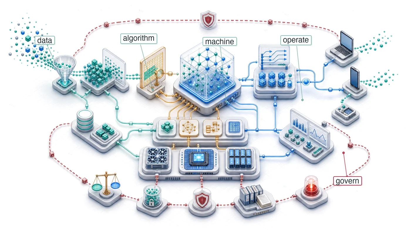
Một quyết định trong môi trường sản xuất có thể đi qua toàn bộ stack. Một pipeline dữ liệu quyết định sự kiện nào được tính là tín hiệu huấn luyện; tín hiệu đó định hình kiến trúc có thể học được tác vụ; kiến trúc xác định dấu chân bộ nhớ và cường độ tính toán số học; những thuộc tính đó giới hạn lựa chọn phần cứng, chiến lược lượng tử hoá, độ trễ phục vụ (serving), giám sát trôi dạt và nghĩa vụ quản trị. Khi nắm vững từng phần riêng lẻ, mỗi lớp là một kỹ năng có giá trị. Khi nắm vững đồng thời, chúng cho khả năng suy luận xuyên các ranh giới. Một kỹ sư chỉ hiểu về nén có thể thu nhỏ một mô hình, nhưng không thể dự đoán việc mất độ chính xác có quan trọng với ngữ cảnh triển khai hay không. Một kỹ sư chỉ hiểu về phục vụ (serving) có thể tối ưu hoá độ trễ, nhưng không thể truy ra một suy giảm hiệu suất bắt nguồn từ thay đổi ở pipeline dữ liệu ba giai đoạn trước đó. Kỷ luật của kỹ thuật hệ thống ML là kỷ luật nhìn thấy những kết nối này, nơi tối ưu hoá của nhóm này trở thành ràng buộc của nhóm khác. Các nguyên tắc chi phối những tương tác đó, gồm lan truyền ràng buộc, bức tường bộ nhớ, nghịch đảo huấn luyện-phục vụ, chi phí điều phối, chi phí giao tiếp và chi phí vận hành mô hình định kỳ trong sản xuất, không gắn với bất kỳ framework, thế hệ phần cứng hay họ mô hình cụ thể nào. Công nghệ sẽ thay đổi, nhưng các ràng buộc vật lý và những đánh đổi nền tảng sẽ còn đó. Theo thuật ngữ D·A·M, điều bền vững là khả năng nhìn vào một hệ thống chưa tồn tại và suy luận cách các ràng buộc về dữ liệu, thuật toán và máy của nó sẽ tương tác, các nút thắt cổ chai sẽ xuất hiện ở đâu, và những quyết định thiết kế nào sẽ trở nên không thể đảo ngược. Thói quen tư duy D·A·M về hệ thống thay vì các thành phần là thứ phân biệt một kỹ sư chỉ có thể xây dựng một phần với một người có thể xây dựng cả hệ thống.
Learning Objectives
- Tổng hợp các nguyên tắc cốt lõi của hệ thống ML thành một framework để suy luận về các ràng buộc của Dữ liệu, Thuật toán và Máy.
- Lần theo cách các quyết định về dữ liệu, kiến trúc, nén, phần cứng, phục vụ (serving), vận hành và quản trị lan truyền các ràng buộc xuyên suốt một hệ thống ML
- Áp dụng phương pháp suy luận theo mô hình hải đăng để chẩn đoán các nút thắt cổ chai trong các kịch bản triển khai trên đám mây, di động, edge, khuyến nghị và TinyML
- Đánh giá các đánh đổi khi triển khai bằng cách xem xét ngân sách độ trễ, việc di chuyển dữ liệu trong bộ nhớ, hiện tượng trôi dạt (drift), trách nhiệm và các ràng buộc về tính bền vững
- Thiết kế một cách tiếp cận kỹ thuật hệ thống cho các ngữ cảnh mới nổi, trước khi chi phí điều phối ở quy mô đội hình trở nên áp đảo
Tổng hợp các hệ thống ML
Hãy tưởng tượng bạn triển khai một mô hình phân loại hình ảnh mới cho hàng loạt thiết bị di động. Nhóm kiến trúc đã chọn các tích chập phân tách theo chiều sâu để đạt hiệu quả. Nhóm nén đã lượng tử hoá thành INT8 để tăng tốc độ. Nhóm phục vụ (serving) đã đạt mục tiêu độ trễ p99 là 50 ms. Mỗi nhóm đều thành công theo tiêu chí riêng của mình, nhưng chỉ trong vài tuần, người dùng bắt đầu phàn nàn: độ chính xác đã giảm bốn điểm phần trăm trên các nhóm firmware và thiết bị cụ thể. Nguyên nhân là do sự tương tác tinh tế giữa lược đồ lượng tử hoá và một nhánh tiền xử lý hình ảnh đặc thù của firmware. Không có thành phần nào tự nó bị hỏng, nhưng pipeline dữ liệu, kiến trúc, chiến lược nén, phần cứng mục tiêu và hạ tầng giám sát đã gắn kết với nhau trong môi trường sản xuất.
Kỹ thuật có trách nhiệm không phải là một lớp bên ngoài được thêm vào sau khi tối ưu hoá, mà là kỷ luật của việc đặc tả, kiểm thử, giám sát và quản trị toàn bộ hệ thống. Bài học đó giờ đây được khái quát hoá trên toàn bộ phần nền tảng này. Hệ thống ML là một bài toán kỹ thuật khác với phần mềm truyền thống vì mô hình không thể tách rời khỏi hệ thống sản xuất, phục vụ và giám sát nó.
Cuốn sách bắt đầu với định luật sắt của hệ thống ML (nguyên tắc 3). Ba thành phần của định luật—di chuyển dữ liệu, tính toán và chi phí phụ trợ—từng có vẻ trừu tượng, nay là các đòn bẩy kỹ thuật chính để phân tích định lượng những hệ thống vốn mơ hồ trước đây. Xây dựng trí tuệ đòi hỏi cả thuật toán và sự tuân thủ hợp đồng silicon (nguyên tắc 4), tức thoả thuận vật lý và kinh tế giữa mô hình và máy. Cường độ số học và suy luận roofline giúp biến những trực giác mơ hồ về hiệu năng thành các quyết định kỹ thuật định lượng (Williams et al. 2009).
Nền tảng định lượng dẫn đến một nhận định rộng hơn: những thành tựu hiện đại của trí tuệ nhân tạo là kết quả tổng hòa từ sự đồng thiết kế D·A·M, chứ không phải do bất kỳ một phát kiến thuật toán đơn lẻ nào. Machine learning thuộc cùng truyền thống kỹ thuật đã tạo ra những máy tính đáng tin cậy, nơi các năng lực mới xuất hiện nhờ sự phối hợp chặt chẽ của nhiều thành phần. Kiến trúc transformer đã giới thiệu một họ mô hình dựa trên cơ chế chú ý (Vaswani et al. 2017), và sau đó các hệ thống mô hình ngôn ngữ lớn như GPT-3 và Llama 2 đã cho thấy cách họ mô hình này mở rộng để trở thành một khối lượng công việc (workload) trung tâm cho các hệ thống ML hiện đại (Brown et al. 2020; Touvron et al. 2023). Bản thân thiết kế toán học của nó không đủ để giải thích giá trị thực tiễn. Giá trị đó phụ thuộc vào việc tích hợp các cơ chế chú ý với hạ tầng huấn luyện phân tán, các kỹ thuật tối ưu hóa hiệu quả bộ nhớ, và các framework vận hành đáng tin cậy.
Việc tích hợp mang lại những hệ quả cụ thể. Chúng ta thường xem “mô hình” là một tệp trọng số, một khối 500 MB gồm các số dấu phẩy động. Tuy nhiên, trong môi trường sản xuất, các trọng số chỉ là một thành phần của mô hình thực sự, và thường không phải là thành phần quan trọng nhất. Một mô hình có thể đưa ra dự đoán hoàn hảo nhưng sẽ vô dụng nếu nhận đầu vào bị lỗi, và một mô hình được huấn luyện trơn tru cũng sẽ thất bại nếu không thể triển khai một cách đáng tin cậy. Mô hình thực sự là tổng hòa của pipeline dữ liệu định nghĩa những gì mô hình nhìn thấy, hạ tầng huấn luyện quyết định những gì nó học được, hệ thống phục vụ (serving) quyết định cách nó tương tác với thế giới, và vòng lặp giám sát giúp nó bám sát thực tế. Tối ưu hóa hệ thống thì mô hình sẽ cải thiện. Bỏ bê hệ thống thì mô hình sẽ suy giảm. Kỹ thuật hệ thống không phải là một phần bổ trợ cho ML; nó chính là sự triển khai của ML. Hệ thống chính là mô hình.
Checkpoint 1.1: Tư duy hệ thống
Các phụ thuộc, vòng lặp phản hồi và đường dẫn yêu cầu của hệ thống khiến ranh giới của nó có thể kiểm thử.
Sự tích hợp
Tính tổng thể
Việc theo dõi một yêu cầu từ đầu đến cuối, như checkpoint yêu cầu, cũng nhấn mạnh cùng một luận điểm ở cấp độ cấu trúc: ranh giới hệ thống định nghĩa khả năng của mô hình. Nhận định này đã dẫn dắt toàn bộ hành trình khám phá trong cuốn sách. Chúng ta bắt đầu bằng cách làm rõ nền tảng: kỹ thuật dữ liệu (Kỹ thuật dữ liệu) và lựa chọn dữ liệu (Lựa chọn dữ liệu) quyết định hệ thống có thể học gì; tính toán thần kinh (Tính toán nơ-ron) và kiến trúc mạng (Kiến trúc mạng) quyết định tín hiệu đó được biến thành tính toán như thế nào; còn các hệ thống huấn luyện (Huấn luyện mô hình) và các framework (Các Framework ML) biến phần tính toán đó thành một quá trình tối ưu hóa có thể thực thi.
Khi nền tảng đã được thiết lập, bài toán kỹ thuật chuyển từ xây dựng sang thương lượng lại các ràng buộc. Nén mô hình (Nén mô hình) làm thay đổi sự đánh đổi giữa độ chính xác, bộ nhớ và độ trễ; tăng tốc phần cứng (Tăng tốc phần cứng) kiểm tra liệu phép tính kết quả có thực sự chạy được trên silicon hay không; và benchmarking (Benchmarking) cung cấp kỷ luật đo lường cần thiết để phân biệt tăng tốc thực sự với hiệu ứng giả. Môi trường sản xuất sau đó phơi bày những giả định vượt qua được phòng thí nghiệm nhưng thất bại dưới tải: các hệ thống phục vụ (serving) (Phục vụ mô hình) phải đáp ứng ngân sách độ trễ, các thực hành vận hành (Vận hành machine learning) phải giữ mô hình ở trạng thái khỏe mạnh khi phân phối thay đổi, và kỹ thuật có trách nhiệm (Kỹ thuật có trách nhiệm) phải đánh giá hệ thống phục vụ ai và ở đâu hiệu suất tổng thể che khuất thất bại của các nhóm nhỏ. Các chương này hoàn thiện khuôn khổ năm trụ cột ở phần mở đầu: kỹ thuật dữ liệu, hệ thống huấn luyện, hạ tầng triển khai, vận hành và giám sát, và trụ cột đạo đức - quản trị được lồng ghép xuyên suốt Phần IV thay vì tách riêng.
Mỗi chương đóng góp một mảnh ghép. Tuy nhiên, bài học thực sự không nằm ở từng mảnh ghép riêng lẻ, mà ở cách chúng tương tác và ràng buộc lẫn nhau. Một lựa chọn kiến trúc có thể mở đường cho một lựa chọn nén, từ đó cho phép một lựa chọn tăng tốc, định hình một ràng buộc về phục vụ (serving) và xác định một yêu cầu vận hành. Chẳng hạn, thiết kế phân tách theo chiều sâu của MobileNetV2 hướng đến suy luận thị giác hiệu quả trên thiết bị di động (Sandler et al. 2018), trong khi lượng tử hoá số học số nguyên đã biến việc triển khai INT8 thành một lộ trình suy luận thực tế (Jacob et al. 2018). Sự kết hợp này có thể giúp triển khai NPU di động, định hình ràng buộc độ trễ p99 và đòi hỏi giám sát trôi dạt trên các tập thiết bị đa dạng. Mọi quyết định đều lan truyền về sau, và một kỹ sư chỉ hiểu một lớp sẽ khó dự đoán những thay đổi sẽ ảnh hưởng đến các phần còn lại như thế nào.

Các lựa chọn kiến trúc gây hiệu ứng dây chuyền đến nén, phục vụ (serving), trôi dạt và quản trị.
Các mô hình hải đăng cung cấp một bản đồ ràng buộc, giúp chúng ta suy luận về các hệ thống ML như một tổng thể thay vì chỉ là tập hợp các bộ phận. Chúng lần theo các tương tác tương tự xuyên suốt các chương, trước khi phần tổng hợp chính thức hoá 13 nguyên tắc định lượng — bao gồm các giới hạn chính xác và các mô hình chẩn đoán phụ thuộc vào giả định — để suy luận về hành vi của hệ thống ML. Sau đó, các nguyên tắc này được mang vào ba lĩnh vực ứng dụng, các hướng phát triển tương lai nơi tư duy hệ thống sẽ quan trọng nhất, và trách nhiệm kỹ thuật đi kèm khi xây dựng những hệ thống mạnh mẽ như vậy.
Các mô hình hải đăng: Lan truyền ràng buộc
Năm mô hình hải đăng được giới thiệu trong Định luật sắt của hệ thống ML đã giúp cụ thể hoá sự lan truyền ràng buộc này, đóng vai trò như những công cụ khám phá hệ thống xuyên suốt cuốn sách. Mỗi mô hình đã chỉ ra cách các khối lượng công việc (workload) khác nhau làm lộ các nút thắt khác nhau.
Năm khối lượng công việc (workload) hải đăng làm nổi bật các nhóm ràng buộc đặc trưng:
- ResNet-50: Kích thước batch có thể chuyển suy luận hình ảnh từ bị giới hạn bởi bộ nhớ sang bị giới hạn bởi thông lượng tính toán.
- GPT-2/Llama: Giải mã tự hồi quy với batch thấp thường bị giới hạn bởi băng thông bộ nhớ vì mỗi bước tái sử dụng trọng số quá ít. Batching, prefill, kiến trúc, song song hoá và phần cứng có thể dịch chuyển nút thắt này.
- MobileNetV2: Các tích chập phân tách theo chiều sâu và lượng tử hoá INT8 đánh đổi bớt khả năng biểu diễn để có thể triển khai trên NPU di động trong bối cảnh bị giới hạn công suất.
- DLRM: Các bảng embedding ở quy mô terabyte có thể khiến dung lượng bộ nhớ trở thành một ràng buộc chặt, song hành với băng thông bộ nhớ. Điều này buộc kỹ sư phải thiết kế xoay quanh nơi dữ liệu nằm trên phần cứng và cách các phép toán thưa vận hành.
- Phát hiện từ khóa (KWS)/Wake Vision: Với các mô hình vi điều khiển dưới 1 megabyte và suy luận luôn bật trong ngân sách công suất tính bằng miliwatt, từng byte và từng miliwatt đều trở nên cực kỳ quan trọng.
Tổng hợp lại, năm khối lượng công việc (workload) này bao quát phổ triển khai từ trung tâm dữ liệu đến vi điều khiển, giúp chúng ta nhận diện các nút thắt mà các nguyên tắc đã chẩn đoán và thử nghiệm các chiến lược tối ưu hoá được phát triển xuyên suốt cuốn sách. Tư duy hệ thống mà chúng tôi xây dựng bằng cách theo dõi các “mô hình hải đăng” này qua từng chương — từ thiết kế kiến trúc, huấn luyện, tối ưu hoá đến triển khai — là góc nhìn tích hợp giúp phân biệt kỹ thuật hệ thống ML với việc phát triển thuật toán đơn lẻ.
Table 1 minh hoạ hành trình này cho một mô hình cụ thể là MobileNetV2, cho thấy các nguyên tắc từ khắp cuốn sách hội tụ như thế nào vào một sản phẩm kỹ thuật. Bảng này đi qua bảy giai đoạn (từ các ràng buộc cơ bản, kiến trúc, huấn luyện, nén, tăng tốc, phục vụ (serving) đến vận hành), qua đó chỉ ra cách các quyết định ở mỗi giai đoạn lan sang và định hình những gì có thể đạt được ở các giai đoạn tiếp theo.
| Giai đoạn Hành trình | Góc nhìn Hệ thống | Triển khai MobileNetV2 |
|---|---|---|
| Nền tảng (Giới thiệu) | Bộ ba AI | Bị giới hạn bởi các ràng buộc của máy (Pin/Nhiệt) |
| Kiến trúc (Kiến trúc mạng) | Hiệu quả thuật toán | Tích chập tách sâu: 8.7× ít FLOPs hơn cho một lớp 3x3, 256 kênh đầu ra đại diện và 13.7× ít phép toán hơn so với ResNet-50 ở quy mô ImageNet |
| Huấn luyện (Huấn luyện mô hình) | Thông lượng so với Độ trễ | Tối ưu hóa cho độ trễ di động một yêu cầu; tăng cường dữ liệu có thể cải thiện độ bền vững |
| Nén (Nén mô hình) | Điều hướng Biên Pareto | Lượng tử hoá INT8: FP32 sử dụng 4× và FP16 sử dụng 2× dung lượng lưu trữ trên mỗi giá trị của INT8, với độ chính xác được xác thực lại theo từng triển khai |
| Tăng tốc (Tăng tốc phần cứng) | Tôn trọng Hợp đồng Silicon | Ánh xạ các kernel đến các NPU di động (ví dụ, Apple Neural Engine) để tối đa hóa việc sử dụng phần cứng |
| Phục vụ (serving) (Phục vụ mô hình) | Tôn trọng Ngân sách Độ trễ | Ràng buộc \(\text{p99} < 50\) ms; tối ưu hóa tiền xử lý (thay đổi kích thước/chuẩn hóa) để tránh tắc nghẽn CPU |
| Vận hành (Vận hành machine learning) | Quản lý Entropy Hệ thống | Giám sát trôi dạt: Phát hiện sự dịch chuyển phân phối và theo dõi độ chính xác cấp độ nhóm trên các quần thể thiết bị không đồng nhất và điều kiện ánh sáng |
Bảng này cho thấy quyết định ở một hàng sẽ ràng buộc các lựa chọn ở hàng kế tiếp như thế nào. Chẳng hạn, lựa chọn về kiến trúc (tích chập tách biệt theo chiều sâu) cho phép các lựa chọn nén (lượng tử hoá INT8), và từ đó mở đường cho các lựa chọn tăng tốc (triển khai trên NPU di động). Việc các ràng buộc lan truyền qua nhiều bước là điều thường thấy trong các hệ thống ML, và hành trình của MobileNetV2 là một ví dụ. Câu hỏi là những công cụ định lượng nào lặp lại giữa các mô hình và công nghệ cụ thể. Câu trả lời nằm ở mười ba nguyên tắc định lượng, gồm cả các giới hạn chính xác và các phép chẩn đoán phụ thuộc vào giả định.
Self-Check: Question
A production image classifier deployed across a mobile device fleet shows a 4-percentage-point drop in accuracy on specific handset cohorts. The weights file is unchanged, the compression team verified INT8 kernel speedups, and the serving team confirmed a P99 latency of 48 ms (under the 50 ms SLO). Which diagnostic posture is most consistent with the ‘system is the model’ thesis?
- Focus the investigation exclusively on serving execution, because runtime inference is the only stage operating during production.
- Trace the interaction between INT8 quantization scaling factors and firmware-specific image preprocessing paths, because production behavior is defined by the weights combined with the data pipeline, runtime hardware, and monitoring loop.
- Escalate to the architecture team to train wider convolutional layers, because an unchanged weights file implies that any remaining error must stem from model capacity.
- Treat the 4-point regression as acceptable random noise, because all engineering teams independently satisfied their local component metrics and the aggregate P99 latency is within budget.
A production recommender workload is dominated by terabyte-scale embedding tables where engineers spend significant effort deciding where data physically resides across storage tiers rather than optimizing dense matrix math. Which Lighthouse model embodies this constraint regime, and how does its primary bottleneck differ from low-batch GPT-2/Llama decoding?
- MobileNetV2; it is capacity-bound on microcontrollers, whereas autoregressive decoding is latency-bound by network packet round-trip times.
- ResNet-50; it is capacity-bound by image batch activation footprints in host DRAM, whereas LLM decode is compute-bound.
- Keyword Spotting (KWS); it is capacity-bound by microcontroller flash storage, whereas LLM decode is strictly compute-bound by tensor core peak FLOP/s.
- DLRM; it is capacity-bound by terabyte-scale embedding tables requiring physical data placement design, whereas low-batch LLM decode is memory-bandwidth-bound due to streaming weights with minimal arithmetic reuse per token.
Order the following phases of the MobileNetV2 Lighthouse Journey in their chronological lifecycle order as constraints propagate from initial requirements through deployment operations:
- Compression (INT8 quantization navigating the Pareto frontier)
- Acceleration (Mapping operators to mobile NPUs under the Silicon Contract)
- Foundations (Establishing battery, thermal, and machine constraints)
- Architecture (Depthwise separable convolutions reducing FLOPs)
- Operations (Cohort-level drift monitoring across heterogeneous devices)
- Serving (Enforcing P99 latency budgets under 50 ms)
True or False: If every engineering team in an ML organization independently satisfies its isolated component metric (e.g., architecture achieves an \(8.7\times\) FLOP reduction, compression achieves \(4\times\) weight reduction, and serving meets its P99 latency SLO), the integrated system is mathematically guaranteed to meet its end-to-end accuracy and correctness requirements in production.
The conclusion argues that ‘the system is the model.’ Explain why treating the model solely as a static weights file (e.g., a 500 MB floating-point binary) fails in production, and define what constitutes the ‘true model.’
Mười Ba Nguyên Tắc Định Lượng
Xuyên suốt cuốn sách này, mỗi phần đều giới thiệu các công cụ định lượng để phân tích hành vi của hệ thống ML. Mười ba nguyên tắc định lượng này được tổng hợp có chủ đích, kết hợp các giới hạn toán học chính xác, các phân tách kỹ thuật, các mô hình cục bộ được khớp, các yêu cầu về chính sách và các phương pháp heuristic trong thiết kế. Table 2 tổng hợp cả mười ba nguyên tắc vào một chỗ, được sắp xếp theo bốn phần đã hé lộ chúng. Giá trị của chúng nằm ở việc áp dụng từng nguyên tắc trong phạm vi các giả định đã nêu, chứ không phải coi mỗi hàng là một định luật phổ quát.
| # | Nguyên tắc | Phần | Phương trình/Tuyên bố cốt lõi | Điều nó dự đoán |
|---|---|---|---|---|
| 1 | Nguyên tắc Dữ liệu là Mã | I: Nền tảng | Behavior \(=f\)(data, algorithm, code, randomness) | Dữ liệu thay đổi hành vi; các đầu vào khác cũng quan trọng |
| 2 | Nguyên tắc Trọng lực Dữ liệu | I: Nền tảng | Di chuyển tính toán về phía dữ liệu khi chi phí truyền tải lặp lại vượt quá chi phí đặt chỗ | Phụ thuộc vào khối lượng, tái sử dụng, mạng và khả năng di chuyển của tính toán |
| 3 | Luật Sắt của Hệ thống ML | II: Xây dựng | \(T_{\text{seq}}=D_{\text{vol}}/\text{BW}+O/(R_{\text{peak}}\eta_{\text{hw}})+L_{\text{lat}}\); sự chồng chéo dao động từ tối đa đến tổng | Các giai đoạn có thể cộng thêm hoặc chồng chéo |
| 4 | Hợp đồng Silicon | II: Xây dựng | \(I_{\text{ridge}}=R_{\text{peak}}/\text{BW}\); so sánh \(I_{\text{model}}\) với \(I_{\text{ridge}}\) | Chẩn đoán hoạt động bị giới hạn bởi băng thông so với tính toán |
| 5 | Biên Pareto | III: Tối ưu hóa | \(\nexists c'\ne c:\,[\forall k\,M_k(c')\ge M_k(c)]\land[\exists j\,M_j(c')>M_j(c)]\) | Không có cấu hình riêng biệt nào chiếm ưu thế tại một điểm biên |
| 6 | Định luật Cường độ Số học | III: Tối ưu hóa | \(R_{\text{attain}} \le \min(R_{\text{peak}},\; I \times \text{BW})\) | Nhiều tính toán hơn không thể nâng cao giới hạn băng thông |
| 7 | Bất biến Năng lượng-Chuyển động | III: Tối ưu hóa | \(E_{\text{total}}=\sum_j N_jE_j\); tỷ lệ chi phí DRAM/FLOP: 173–582× | Tổng năng lượng phụ thuộc vào số lượng và chi phí sự kiện |
| 8 | Định luật Amdahl | III: Tối ưu hóa | \(\text{Speedup} = \frac{1}{(1-f_{\text{parallel}}) + \frac{f_{\text{parallel}}}{S_{\text{parallel}}}}\) | Phần tuần tự giới hạn tất cả các lợi ích song song |
| 9 | Khoảng cách Xác minh | IV: Triển khai | \(\Pr_{(X,Y)\sim P_{\text{deploy}}}[d(f(X),Y)\le\tau]\ge1-\epsilon\) | Chỉ định khoảng cách, dung sai, quần thể và độ tin cậy |
| 10 | Chẩn đoán Trôi dạt Thống kê | IV: Triển khai | \(\text{Accuracy}(t)\approx\text{Accuracy}_0-\lambda\mathcal{D}(P_t\Vert P_0)\) | Một sự phù hợp cục bộ; sự trôi dạt không nhất thiết làm giảm chất lượng |
| 11 | Chẩn đoán Lệch Huấn luyện-Phục vụ | IV: Triển khai | \(S_{\text{skew}}=\mathbb{E}_{X\sim P_{\text{deploy}}}[d(f_{\text{serve}}(X),f_{\text{train}}(X))]\) | Sự không khớp đầu ra báo hiệu rủi ro, không phải mất độ chính xác |
| 12 | Nguyên tắc Ngân sách Độ trễ | IV: Triển khai | \(T_q\le L_{\text{budget}}\) | SLO của sản phẩm chọn \(q\) và ngân sách của nó |
| 13 | Mô hình Phản hồi Độ chệch (Bias) | IV: Triển khai | \(\Delta_g(k)\approx\Delta_g(0)\alpha_{\text{fb}}^k\) với \(\alpha_{\text{fb}}\) đã được khớp | Phản hồi có thể khuếch đại tác hại; đo lường và can thiệp |
Mười ba nguyên tắc này không phải là các tiên đề độc lập. Chúng tạo thành một framework tích hợp, được kết nối bởi một siêu nguyên tắc duy nhất: heuristic bảo toàn độ phức tạp.1 Khi giảm bớt độ phức tạp ở một giao diện, nó thường sẽ xuất hiện lại ở phần khác của hệ thống. Tuy nhiên, đây không phải là một định luật bảo toàn vật lý và không hàm ý rằng mọi sự đơn giản hoá đều phải có một chi phí bù đắp tương xứng. Giá trị của heuristic này nằm ở tính chẩn đoán: sau khi đơn giản hoá một thành phần, hãy kiểm tra xem gánh nặng về xác thực, trạng thái, phối hợp hoặc vận hành đã chuyển dịch ở đâu. Tiêu chí kiểm tra là: các nguyên tắc có giải thích được cùng những điểm nghẽn then chốt từ góc nhìn dữ liệu, mô hình, phần cứng và triển khai mà không mâu thuẫn nhau hay không.
1 Heuristic bảo toàn độ phức tạp: Định luật Tesler, một châm ngôn thiết kế, nói rằng độ phức tạp không thể giảm bớt của một ứng dụng phải được xử lý ở đâu đó trong tương tác giữa người dùng, ứng dụng và nền tảng (Tesler 1984); việc mở rộng điều này cho toàn bộ độ phức tạp của hệ thống ML là một phép loại suy, không phải một định luật vật lý. Lượng tử hoá có thể làm tăng gánh nặng xác thực, và sự trừu tượng hoá có thể đẩy chi tiết triển khai ra sau một giao diện, nhưng thiết kế tốt cũng có thể loại bỏ hẳn độ phức tạp ngẫu nhiên. Các pipeline ứng dụng mô hình ngôn ngữ lớn minh hoạ một sự chuyển dịch có thể xảy ra: đơn giản hoá giao diện người dùng bằng các lời nhắc ngắn hơn hoặc mơ hồ hơn có thể chuyển phần việc sang lời nhắc hệ thống, truy xuất hoặc xác minh đầu ra. Hãy dùng heuristic này để tìm kiếm các chi phí bị dịch chuyển, chứ không mặc định rằng luôn phải tồn tại một chi phí bù đắp tương xứng.
Nền tảng: Nơi độ phức tạp bắt nguồn (nguyên tắc 1–2)
Nguyên tắc dữ liệu như mã (1) và heuristic trọng lực dữ liệu (nguyên tắc 2), được trình bày trong Phần I và phát triển thêm ở Kỹ thuật dữ liệu, xem dữ liệu là một đầu vào logic quan trọng và một điểm neo vật lý tiềm năng. Hành vi cũng phụ thuộc vào thuật toán và cách triển khai. Việc đưa tính toán tới dữ liệu phụ thuộc vào khối lượng, mức tái sử dụng, chi phí mạng và khả năng di động của phần tính toán. Vì vậy, hành vi và kiến trúc của mô hình sẽ kế thừa các ràng buộc từ nền dữ liệu.
Các mô hình hải đăng minh họa trực tiếp cả hai nguyên tắc này. ResNet-50 và GPT-2 phụ thuộc vào cả kiến trúc và dữ liệu huấn luyện của chúng. Với DLRM, các bảng embedding quy mô terabyte cho thấy rõ rằng hệ thống cần được thiết kế xoay quanh nơi dữ liệu nằm ở đâu về mặt vật lý. Những nguyên tắc này giúp giải thích vì sao mẫu bố trí đưa tính toán tới dữ liệu lặp lại trong nhiều bối cảnh triển khai, nhưng không biến nó thành một quy tắc đặt vị trí mang tính phổ quát.
Xây dựng: Độ phức tạp biến thành tính toán như thế nào (nguyên tắc 3–4)
Luật sắt (nguyên tắc 3) và hợp đồng silicon (nguyên tắc 4) là kim chỉ nam cho các quyết định khi xây dựng một hệ thống ML. Việc phân rã ba thành phần của luật sắt (được giới thiệu trong Định luật sắt của hệ thống ML) chỉ ra nên tác động vào yếu tố nào; còn hợp đồng silicon xác định thành phần nào chiếm ưu thế đối với một cặp kiến trúc-phần cứng cụ thể. Như hành trình hải đăng đã cho thấy, mỗi mô hình có thể bộc lộ những chế độ giới hạn khác nhau: suy luận ResNet-50 theo batch có thể bị giới hạn bởi khả năng tính toán, giải mã Llama với batch nhỏ có thể bị giới hạn bởi băng thông, DLRM có thể bị giới hạn bởi dung lượng, và MobileNetV2 điều chỉnh cách tính toán để phù hợp với các giới hạn của NPU di động. Chẩn đoán nút thắt cổ chai liên hệ từng chế độ này với các tối ưu hóa đem lại hiệu quả và những cách tiếp cận lãng phí công sức, biến việc chẩn đoán xem hệ thống bị giới hạn bởi tính toán, băng thông hay dung lượng thành một kế hoạch hành động cụ thể. Huấn luyện mô hình xác nhận rằng thời gian huấn luyện giảm mạnh nhất khi các kỹ sư tối ưu hóa yếu tố chiếm ưu thế, thay vì phân bổ công sức đồng đều.
Tối ưu hóa: Các ràng buộc định hình sự đánh đổi như thế nào (nguyên tắc 5–8)
Bốn nguyên tắc tối ưu hoá này tạo thành một chuỗi chẩn đoán liên kết chặt chẽ. Biên Pareto (nguyên tắc 5) xác định các đánh đổi không bị chi phối sau khi hướng mục tiêu được chuẩn hoá: lượng tử hoá đánh đổi độ chính xác lấy lưu lượng truy cập bộ nhớ; tỉa (pruning) đánh đổi dung lượng mô hình lấy tốc độ; và chưng cất (distillation) đánh đổi chi phí tính toán khi huấn luyện lấy hiệu quả suy luận. Định luật cường độ số học (nguyên tắc 6) chẩn đoán liệu tính toán hay băng thông là trần lý tưởng. Bất biến năng lượng-chuyển động (nguyên tắc 7) kết hợp chi phí trên mỗi sự kiện với số lượng sự kiện: trong các hằng số tham chiếu của sách, một lần truy cập DRAM tốn khoảng 173–582× năng lượng so với một phép toán số học FP32/FP16, nhưng mức chi phối tổng thể của khối lượng công việc (workload) còn phụ thuộc vào tần suất của từng loại sự kiện. Định luật Amdahl (nguyên tắc 8) đặt trần cho mọi lợi ích từ song song hoá, giải thích vì sao tải dữ liệu và tiền xử lý có thể trở thành nút thắt cổ chai trong các hệ thống đã tối ưu hoá cao.
MobileNetV2 (mô hình mẫu của chúng ta từ Kiến trúc mạng) điều hướng đồng thời cả bốn nguyên tắc: tích chập tách chiều sâu định hình lại biên Pareto (Sandler et al. 2018); lượng tử hoá INT8 khai thác định luật cường độ số học bằng cách tăng số phép toán trên mỗi byte nhờ giảm lưu lượng truy cập bộ nhớ (Jacob et al. 2018); và mức tiết kiệm năng lượng đạt được vẫn tuân theo bất biến năng lượng-chuyển động, trong khi Định luật Amdahl giải thích vì sao một giai đoạn tiền xử lý chưa được tăng tốc có thể giới hạn tốc độ tăng tốc tổng thể. Mô hình mẫu KWS đẩy những đánh đổi này tới mức cực hạn, nơi các mô hình dưới 1 megabyte trên vi điều khiển không để lại bất kỳ biên độ lãng phí nào ở bất kỳ khía cạnh nào.
Triển khai: Thực tế phá vỡ các giả định (nguyên tắc 9–13)
Các nguyên tắc triển khai nhắm tới những trục trặc mà thử nghiệm nội bộ (bench testing) không thể loại trừ: một hệ thống có thể chạy đúng khi thử nghiệm nhưng lại âm thầm hỏng khi vào sản xuất. Khoảng trống xác minh (nguyên tắc 9) cho thấy xác minh thống kê chỉ có hiệu lực trong một phạm vi được nêu rõ, gồm tập triển khai, mức độ khác biệt của tác vụ, dung sai, sai số mục tiêu và thủ tục ước lượng độ tin cậy với mẫu hữu hạn; thử nghiệm chỉ ước tính hành vi thay vì chứng minh tính đúng đắn cho mọi đầu vào trong tương lai. Công cụ chẩn đoán trôi dạt thống kê (nguyên tắc 10) phát hiện sự thay đổi phân phối nhưng không cho biết độ chính xác đang xấu đi, giữ nguyên hay cải thiện, nên một đường cong suy giảm cục bộ chỉ có ý nghĩa khi được khớp theo các kết quả quan sát. Tương tự, công cụ chẩn đoán độ chệch (skew) giữa huấn luyện và phục vụ (serving) (nguyên tắc 11) cũng là chỉ báo rủi ro chứ không phải phương trình chung cho mức mất độ chính xác, dù khác biệt ở khâu tiền xử lý hoặc số học vẫn có thể làm thay đổi chất lượng. Ngân sách độ trễ (nguyên tắc 12) ràng buộc việc phục vụ (serving) tại phân vị do yêu cầu sản phẩm chọn, như p95, p99, hoặc một thước đo đuôi khác. Cuối cùng, mô hình phản hồi độ chệch (bias) (nguyên tắc 13) có thể biểu diễn hiện tượng khuếch đại chênh lệch, nhưng để xuất hiện một truy hồi theo hàm mũ cần có hệ số phản hồi đã đo lường, xấp xỉ hằng và không có can thiệp hiệu quả.
Năm nguyên tắc triển khai giải thích vì sao Vận hành machine learning dành nhiều công sức cho giám sát, phát hiện drift, kho đặc trưng và các chỉ số tách theo nhóm con: hạ tầng vận hành phải làm lộ những lỗi ngầm và gắn bằng chứng với hành động ứng phó. Một hệ thống đề xuất DLRM dù đạt độ chính xác ngoại tuyến xuất sắc vẫn cần kiểm tra đối sánh khi độ lệch giữa huấn luyện và phục vụ (serving) làm sai lệch giá trị đặc trưng (nguyên tắc 11), và cần kiểm tra kết quả khi hành vi người dùng biến động theo mùa (nguyên tắc 10). Khi phục vụ (serving) các mô hình như GPT-2/Llama, hệ thống phải tuân theo phân vị độ trễ đã chọn bằng các kỹ thuật như ghép batch liên tục và giải mã suy đoán, như trình bày trong Phục vụ mô hình, vì thời gian phản hồi quá lâu có thể vi phạm yêu cầu sản phẩm. Một hệ thống phê duyệt khoản vay có thể đáp ứng mọi nguyên tắc khác nhưng vẫn có thể từ chối cấp tín dụng một cách có hệ thống cho các cộng đồng yếu thế, và vòng phản hồi có thể làm trầm trọng thêm tổn hại trừ khi giám sát theo nhóm con tách riêng phát hiện ra và kích hoạt việc xem xét.
Framework tích hợp
Mười ba nguyên tắc này không phải là một checklist để áp dụng tuần tự. Chúng tạo thành một mạng lưới ràng buộc lẫn nhau. Heuristic “bảo toàn độ phức tạp” nhắc kỹ sư tìm xem việc đơn giản hóa cục bộ đang đẩy gánh nặng sang chỗ khác.
Chúng ta có thể lần theo các ràng buộc qua lại này một cách cụ thể bằng cách xem điều gì xảy ra khi một kỹ sư lượng tử hoá một mô hình từ FP16 xuống INT8. Quyết định đơn lẻ này di chuyển trên biên Pareto (nguyên tắc 5), đánh đổi độ chính xác để giảm lưu lượng bộ nhớ. Hệ quả không dừng ở đó: lượng tử hoá thay đổi “hợp đồng silicon” của mô hình (nguyên tắc 4), dịch chuyển vị trí của nó trên đường cong cường độ tính toán (nguyên tắc 6) và làm thay đổi đặc tính năng lượng của mô hình (nguyên tắc 7). Khi mô hình đã lượng tử hoá được triển khai, ngân sách độ trễ (nguyên tắc 12) quyết định liệu mức tăng tốc có đáp ứng mục tiêu mức dịch vụ (SLO) hay không, trong khi xác thực triển khai phải kiểm tra xem đường dẫn phục vụ (serving) đã lượng tử hoá có giữ nguyên hành vi đã được chấp nhận trong quá trình kiểm thử nén hay không. Một quyết định lượng tử hoá duy nhất sẽ đồng thời gợn sóng qua biên Pareto, hợp đồng silicon và ngân sách độ trễ, nơi một lợi thế ở khía cạnh này (lưu lượng bộ nhớ) phải được kiểm chứng trước rủi ro ở khía cạnh khác (lỗi số học).
Việc theo dõi đó không đòi hỏi tất cả các nguyên tắc cùng áp dụng một lúc. Nó cho thấy các nguyên tắc liên quan sẽ lần lượt trở nên hữu ích khi một quyết định chuyển từ biểu diễn mô hình sang thực thi trên phần cứng rồi đến xác thực trong môi trường sản xuất. Cách bố trí dữ liệu quyết định mô hình có thể chạy ở đâu, Định luật Amdahl giới hạn mức mà một kernel nhanh hơn có thể cải thiện toàn bộ đường dẫn yêu cầu, xác minh đặt giới hạn cho mức mất mát độ chính xác, và giám sát kết quả kiểm tra xem hành vi đã được xác thực có còn duy trì sau khi triển khai hay không. Nhiệm vụ của kỹ sư là lần theo các chi phí bị dịch chuyển, thay vì giả định rằng độ phức tạp được bảo toàn.
Một đề xuất triển khai nhỏ sẽ làm cho mạng lưới các ràng buộc này trở nên cụ thể.
Checkpoint 1.2: Áp dụng các nguyên tắc
Một đồng nghiệp đề xuất lượng tử hoá mô hình của bạn từ FP32 sang INT8 để giảm chi phí phục vụ (serving).
Theo dõi các nguyên tắc
Để thấy rõ chu trình ràng buộc lẫn nhau này, hãy theo dõi luồng trong figure 1. Bốn giai đoạn (Nền tảng, Xây dựng, Tối ưu hoá, Triển khai) bao quanh một trung tâm đại diện cho nguyên tắc heuristic bảo toàn độ phức tạp, và các mũi tên thể hiện luồng các quyết định kỹ thuật: lựa chọn ở mỗi giai đoạn sẽ ràng buộc những gì có thể làm ở giai đoạn tiếp theo, và cuối cùng chu trình quay trở lại điểm xuất phát. Các quyết định trong Xây dựng sẽ ràng buộc Tối ưu hoá, trong khi bằng chứng từ môi trường sản xuất như drift, skew và thay đổi kết quả có thể phản hồi về Nền tảng. Vai trò của kỹ sư là quản lý luồng này, đảm bảo các gánh nặng bị dịch chuyển sẽ được đặt ở nơi có thể xử lý hiệu quả.
Mũi tên phản hồi từ Triển khai về Nền tảng là trung tâm của chu trình này. Các nguyên tắc từ chín đến mười ba chỉ ra những tín hiệu và ràng buộc có thể đòi hỏi một bản phát hành sửa lỗi, phương án dự phòng, dữ liệu mới, huấn luyện lại, hoặc một lượt tối ưu hoá mới. Khi điều đó xảy ra, kỹ sư cần chẩn đoán phản ứng nào phù hợp với nguyên nhân, thay vì chỉ tự động phản ứng với cảnh báo drift. Chu trình này hoạt động trong phạm vi một hệ thống đơn lẻ mà cuốn sách này đề cập: mục tiêu không phải là đặt tên cho mọi kiến trúc tương lai, mà là giúp phản hồi được nhận biết đủ sớm để kỹ sư có thể thiết kế lại trước khi các lỗi tích tụ.

Theo dõi một đề xuất lượng tử hoá qua bốn nguyên tắc là một lượt chẩn đoán; cách làm tương tự cũng áp dụng khi điểm nghẽn không phải là một đề xuất tối ưu hoá mà là chi phí để phục vụ (serving) một token được sinh ra.
Napkin Math 1.1: Chi phí của một token
Vật lý:
- Tổng dung lượng byte của trọng số mô hình được di chuyển \((D_{\text{vol}})\): 70 billion tham số \(\times\) 2 byte (FP16) = .
- Tính toán \((O)\): \(O \approx 2 \times P =\) 140 GFLOP mỗi token, trong đó \(P\) là số lượng tham số.
- Phần cứng: Hai H100 với băng thông tổng hợp \(\text{BW}\) = 6.70 TB/s, \(R_{\text{peak}} \approx\) 1978 TFLOP/s FP16.
Toán học:
- Thời gian di chuyển dữ liệu: \(T_{\text{mem}} = \frac{140 \text{ GB}}{6700 \text{ GB/s}} \approx 20.9 \text{ ms}\)
- Thời gian tính toán: \(T_{\text{comp}} = \frac{140 \times 10^9 \text{ FLOP}}{1978 \times 10^{12} \text{ FLOP/s}} \approx 0.07 \text{ ms}\)
Nhận định về hệ thống:
Cận dưới lý tưởng cho thời gian truyền qua bộ nhớ \(T_{\text{mem}}\) lớn hơn 295.2× lần so với cận dưới cho thời gian tính toán đỉnh \(T_{\text{comp}}\). Trong mô hình batch kích thước 1 này, giải mã bị giới hạn nặng bởi băng thông (mật độ tính toán \(\approx 1\) FLOP/byte). Dùng batch có thể tăng mức tái sử dụng, còn lượng tử hoá có thể giảm lượng dữ liệu trọng số phải truyền. Chỉ tối ưu phần thực thi tính toán có thể kéo thời gian tính toán thực tế xuống gần cận dưới 0.07 ms, nhưng không thể làm giảm cận dưới thời gian truyền qua bộ nhớ 20.9 ms.
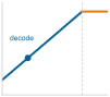
Trong mô hình cận dưới với batch kích thước 1 này, giải mã nằm bên trái sườn roofline, trong vùng bị băng thông chi phối.
Tính toán này cho thấy framework hoạt động như một công cụ chẩn đoán hơn là một hệ thống phân loại trừu tượng. Các chương đã áp dụng những cận dưới, mô hình và heuristic này vào các quyết định kỹ thuật cụ thể, nhiều khi không nêu tên rõ ràng. Lần theo các ứng dụng đó qua ba lĩnh vực—xây dựng nền tảng, kỹ thuật để mở rộng quy mô và điều hướng thực tế sản xuất—cho thấy framework đã dẫn dắt việc phân tích xuyên suốt cuốn sách như thế nào.
Self-Check: Question
Consider serving one token at batch size 1 from a 70-billion-parameter Llama 2 model in FP16 (\(D_{\text{vol}} = 140\text{ GB}\), \(O \approx 140\text{ GFLOP}\)) sharded across two NVIDIA H100 GPUs (aggregate \(\text{BW} = 6.70\text{ TB/s}\), aggregate \(R_{\text{peak}} = 1,978\text{ TFLOP/s}\)). What are the idealized lower bounds for memory transfer (\(T_{\text{mem}}\)) and peak compute (\(T_{\text{comp}}\)), and what systems optimization strategy does this diagnostic dictate?
- Memory transfer time \(T_{\text{mem}} \approx 0.07\text{ ms}\) and compute time \(T_{\text{comp}} \approx 20.9\text{ ms}\); because compute time dominates by \(295\times\), the engineering team should prioritize hand-tuning tensor core matrix multiplication kernels.
- Memory transfer time \(T_{\text{mem}} \approx 2.09\text{ ms}\) and compute time \(T_{\text{comp}} \approx 2.09\text{ ms}\); because the workload operates exactly at the roofline ridge point, compute optimizations and memory optimizations provide identical returns.
- Memory transfer time \(T_{\text{mem}} \approx 20.9\text{ ms}\) and compute time \(T_{\text{comp}} \approx 0.07\text{ ms}\); because the memory bound is \(\approx 295\times\) larger than the compute bound, decode is heavily bandwidth-bound, meaning kernel FLOP tuning yields negligible speedup while batching and quantization directly reduce latency.
- Memory transfer time \(T_{\text{mem}} \approx 41.8\text{ ms}\) and compute time \(T_{\text{comp}} \approx 0.14\text{ ms}\); because sharding across two GPUs doubles the communication overhead, execution time increases by \(2\times\) relative to a single GPU.
According to the Energy-Movement Invariant (\(E_{\text{total}} = \sum_j N_j E_j\)), accessing off-chip DRAM requires approximately 100 to 1,000 times more energy than executing a single FP16 or FP32 arithmetic operation. What is the direct systems design implication of this physical reality?
- Inference engines should prioritize minimizing total ALU operations above all else, even if intermediate tensors must be repeatedly written to and read from off-chip DRAM.
- Hardware accelerators consume identical energy regardless of whether memory accesses hit on-chip SRAM or off-chip DRAM, because memory controller power is fixed.
- Quantization saves energy exclusively by simplifying ALU multiplication logic, while memory traffic volume has negligible impact on total package power.
- Architectures and runtimes must maximize on-chip data reuse (e.g., via operator kernel fusion, SRAM tiling, and weight quantization), because eliminating off-chip DRAM round-trips yields orders-of-magnitude greater energy savings than reducing arithmetic FLOPs.
True or False: The conservation-of-complexity heuristic is an exact physical conservation law of computer science that proves every simplification in an ML pipeline interface creates an identical, mathematically equal compensating burden in another component.
The thirteen quantitative principles are unified by a central meta-heuristic known as the ____ heuristic, which reminds engineers that simplifying one interface often displaces validation, state, or operational burdens to another part of the system.
In the Cycle of ML Systems diagram (figure 1), the Deploy phase contains an explicit feedback arrow returning to Foundations (Data). Explain what production signals activate this feedback loop and why automated rollback is insufficient when the cause is external statistical drift.
Các nguyên tắc trong thực tiễn
Một nhóm dù thuộc lòng cả mười ba nguyên tắc nhưng không xác định được các giả định của chúng hay áp dụng vào một quyết định triển khai thực tế thì coi như chưa học được gì. Bài kiểm tra này giống nhau ở cả ba lĩnh vực trải dài vòng đời ML: xây dựng nền tảng kỹ thuật, kỹ thuật để mở rộng quy mô và điều hướng thực tế sản xuất. Tư duy hệ thống kết nối những gì phân tích từng thành phần riêng lẻ không thể.
Xây dựng nền tảng kỹ thuật
Nguyên tắc dữ liệu là mã (1) đã định hình Kỹ thuật dữ liệu, gợi lại cách Karpathy nhìn nhận Software 2.0 khi xem tập dữ liệu và kiến trúc mô hình như mã nguồn (Karpathy 2017), đồng thời thừa nhận rằng thuật toán và mã phục vụ (serving) cũng ảnh hưởng đến hành vi. Các nền tảng toán học (Tính toán nơ-ron) làm rõ các mô thức tính toán gắn với hợp đồng silicon: phép nhân ma trận ở lõi của tính toán thần kinh quyết định cường độ số học; vị trí của nó so với điểm ridge của phần cứng giúp chẩn đoán liệu một khối lượng công việc (workload) bị giới hạn bởi băng thông hay bởi năng lực tính toán. Việc lựa chọn framework (Các Framework ML) minh hoạ hệ quả thực tế của hợp đồng silicon: mỗi framework đặt ra các ràng buộc về tối ưu đồ thị, quản lý bộ nhớ, hỗ trợ backend phần cứng và các con đường triển khai còn mở. Một kỹ sư chọn framework mà không cân nhắc những hệ quả đó có thể phát hiện quá muộn rằng lựa chọn của mình đã loại bỏ phương án triển khai hiệu quả nhất.
Các lựa chọn nền tảng (chọn lọc dữ liệu nào, dựa vào các phép toán cơ bản nào, dùng framework nào) sẽ lan sang các quyết định kỹ thuật về sau. Sự lan truyền đó càng lộ rõ khi hệ thống phải mở rộng vượt ra khỏi một máy đơn lẻ, lúc này ba thành phần của định luật sắt được mở rộng từ các đại lượng cấp chip sang các ràng buộc cấp cụm.
Kỹ thuật để mở rộng quy mô
Các hệ thống huấn luyện (Huấn luyện mô hình) cho thấy định luật sắt vận hành ra sao: song song theo dữ liệu có thể giảm thời gian tính toán mỗi bước bằng cách phân tán công việc trên nhiều GPU, dù điều này làm tăng chi phí truyền thông; độ chính xác hỗn hợp (mixed precision) giúp giảm lượng dữ liệu di chuyển khi các tensor được biểu diễn ở FP16 thay vì FP32; và gradient checkpointing đánh đổi việc tính toán lại để lấy dung lượng bộ nhớ. Mỗi kỹ thuật này đều tác động vào một thành phần khác nhau của cùng một phương trình ba yếu tố. Nén mô hình (Nén mô hình) đi thẳng vào biên Pareto: lượng tử hoá INT8 của MobileNetV2 và tỉa (pruning) embedding của DLRM đều đánh đổi một chỉ số lấy một chỉ số khác, trong khi định luật cường độ số học giúp chẩn đoán sự đánh đổi nào sẽ mang lại hiệu quả lớn nhất cho một mục tiêu phần cứng cụ thể.
Tuy nhiên, xây dựng và tối ưu hóa một mô hình chỉ giải được một nửa bài toán kỹ thuật. Nửa còn lại bắt đầu khi mô hình rời cụm huấn luyện và đi vào sản xuất, nơi các yêu cầu thống kê, các phép chẩn đoán đã hiệu chỉnh và các chính sách SLO chi phối hành vi; và những tối ưu hóa từng hiệu quả trên bàn thử phải vượt qua tính khó lường của lưu lượng thực tế.
Ứng phó với thực tế sản xuất
Việc chuyển từ huấn luyện sang suy luận thường kéo theo thay đổi mục tiêu tối ưu: trong khi huấn luyện ưu tiên tối đa hóa thông lượng trong nhiều ngày, suy luận tương tác có thể tối ưu hóa một phân vị độ trễ đuôi cụ thể ở mức mili giây. Ví dụ minh họa dùng độ trễ trung bình 50 ms và p99 là 2.000 ms, tức phân vị đuôi được chọn cao gấp 40\(\times\) trung bình; sản phẩm khác có thể quy định p95, p99.9, hoặc đặt thời hạn riêng theo lớp yêu cầu. Phân tích độ trễ đuôi cho thấy vì sao độ trễ trung bình có thể che giấu các yêu cầu quyết định trải nghiệm người dùng (Dean and Barroso 2013). Trong phục vụ (serving) ML, các spike ở phần đuôi có thể xuất phát từ các lần tạm dừng do garbage collection trong các framework suy luận dựa trên Python, dynamic batching hình thành kém tối ưu khi lưu lượng không đều, hoặc quá trình tạo sinh tự hồi quy khi một prompt hoặc đầu ra dài buộc phải làm nhiều việc hơn hẳn so với một phản hồi ngắn điển hình.
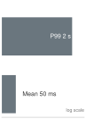
Độ trễ trung bình che giấu độ trễ đuôi; phân vị đuôi được chọn quy định SLO.
Ngoài hiệu suất kỹ thuật, Kỹ thuật có trách nhiệm đã mở rộng framework để bao gồm cả tác động xã hội. Các yêu cầu xác minh thúc đẩy việc giám sát các vi phạm về tính công bằng song song với hiệu suất: theo dõi phân phối dự đoán theo nhóm nhân khẩu học, phát hiện sự khuếch đại độ chệch (bias) theo thời gian (nguyên tắc 13), và cảnh báo khi xuất hiện các chênh lệch độ chính xác không thể giải thích. Giám sát trôi lệch (drift) cũng áp dụng cho phân phối và kết quả của các nhóm con, nơi độ chính xác có thể thay đổi với các nhóm ít được đại diện, ngay cả khi các chỉ số tổng thể vẫn ổn định. Vì vậy, AI có trách nhiệm là một thành phần không thể thiếu của kỹ thuật hệ thống, một ràng buộc thiết kế hàng đầu được quản lý bằng cùng kỷ luật đo lường như hiệu suất.
Ba lĩnh vực này cho thấy mười ba nguyên tắc là những công cụ hữu ích trong thực tế, chứ không phải những tiên đề phổ quát. Câu hỏi bây giờ là ở đâu các giả định của chúng sẽ tiếp tục được kiểm nghiệm, khi các hệ thống ML mở rộng sang các ngữ cảnh triển khai mới, đối mặt với những dạng lỗi mới, và theo đuổi các mục tiêu ngày càng tham vọng.
Self-Check: Question
A team chooses an ML framework primarily for its familiar Python syntax, only to discover months later that deploying the model to mobile NPUs and edge accelerators requires painful manual kernel rewrites because the framework lacks mature compiler lowering and graph optimization for those backends. Why does the Silicon Contract lens classify framework selection as an architectural commitment rather than an ergonomic preference?
- Frameworks embody fundamental architectural commitments to intermediate representations (IR), memory allocators, operator fusion passes, and backend compiler targets, which dictate whether the hardware’s peak efficiency can be realized downstream.
- Standard exchange formats such as ONNX are mathematically guaranteed to recover 100% of native hardware performance regardless of which framework was used during training.
- Frameworks operate exclusively as UI wrappers; hardware execution speed is determined solely by the neural network weights file.
- Modern hardware accelerators execute Python bytecode directly on silicon, so framework differences only affect model training time.
A production serving dashboard for an interactive conversational assistant reports an average (mean) latency of 50 ms. However, user satisfaction metrics are declining, and detailed telemetry reveals a P99 tail latency of 2,000 ms (a \(40\times\) gap over the mean), violating the product SLO (\(T_{0.99} \le 200\text{ ms}\)). Which systems mechanism is a primary root cause of this massive tail spike in ML inference?
- Uniform degradation of memory bus bandwidth across all simultaneous client connections.
- A 40x increase in model weight parameters triggered dynamically whenever traffic surges.
- Heavy-tailed sequence lengths in autoregressive decoding, runtime garbage collection pauses in Python servers, and queueing delays caused by dynamic batching timeouts under bursty request arrivals.
- Deterministic floating-point underflow occurring on exactly one percent of input requests.
True or False: Responsible AI metrics, such as subgroup error rates and bias feedback amplification, can be adequately handled as a post-hoc compliance audit after model serving is fully optimized, because fairness properties remain stable once offline validation passes.
An LLM training run encounters out-of-memory (OOM) errors during long-context training due to massive activation tensor footprints. Explain how Gradient Checkpointing (Activation Recomputation) resolves this bottleneck and identify the explicit systems trade-off it makes.
Contrast the primary optimization objectives and time horizons of ML training systems versus interactive ML inference serving systems.
Định hướng tương lai
Framework này hữu ích nhất khi dự báo được nơi các ràng buộc sẽ bắt đầu “siết” tiếp theo. Ba hướng đang đặt ngày càng nhiều áp lực lên cùng những giới hạn vật lý đó: triển khai trong các ngữ cảnh đa dạng, độ vững dưới điều kiện đối kháng (Goodfellow et al. 2015), và các ứng dụng xã hội mà sai sót của chúng kéo theo hệ quả đối với công chúng. Một hướng thứ tư — các hệ thống ghép nhiều mô hình, công cụ và bộ xác minh, hoặc mở rộng vượt ra ngoài phạm vi một máy — tiếp tục được soi chiếu dưới cùng lăng kính này thay vì thay thế nó.
Áp dụng các nguyên tắc vào các ngữ cảnh triển khai mới
Sự đa dạng trong triển khai kiểm chứng liệu một framework định lượng có thể giải thích các hệ thống với những chế độ tài nguyên tương phản hay không. Đám mây cung cấp công suất dồi dào và phần cứng tập trung, các thiết bị edge và di động vận hành dưới giới hạn về độ trễ và pin, còn TinyML và hệ thống nhúng thì nén cùng một bài toán thiết kế vào vài kilobyte và vài milliwatt. AI tạo sinh không phải là một môi trường triển khai thứ năm; đó là một lớp khối lượng công việc (workload) gây áp lực lên cả bốn môi trường trên.
Trong môi trường đám mây, quyết định then chốt là biến phần cứng dồi dào thành thông lượng hữu ích mà không để việc di chuyển dữ liệu, dung lượng hay chi phí lấn át. Các khối lượng công việc (workload) dày đặc như ResNet-50 theo đuổi việc tận dụng GPU thông qua hợp nhất kernel, huấn luyện với độ chính xác hỗn hợp, và nén gradient; trong khi đó, các hệ thống khuyến nghị kiểu DLRM còn phải quản lý dung lượng và bố trí bảng embedding cùng các mẫu truy cập thưa thớt. Nén mô hình và Huấn luyện mô hình đã khảo sát những kỹ thuật này, cho thấy cách chúng kết hợp để cân bằng tối ưu hiệu năng với hiệu quả chi phí ở quy mô lớn.
Ngược lại, các hệ thống di động và edge phải đối mặt với những giới hạn nghiêm ngặt về công suất, bộ nhớ và độ trễ, nên cần sự đồng thiết kế phần cứng-phần mềm tinh vi. Các kiến trúc hiệu quả trong Kiến trúc mạng (như tích chập phân tách theo chiều sâu và tìm kiếm kiến trúc mạng nơ-ron), kết hợp với các kỹ thuật nén ở Nén mô hình (như lượng tử hoá và tỉa (pruning)), cho phép triển khai trên những thiết bị mà nền tảng di động tham chiếu của sách chỉ có dung lượng bộ nhớ nhỏ hơn khoảng 10× lần và mức công suất nhỏ hơn khoảng 140× lần so với một bộ tăng tốc hạng H100. Việc triển khai edge trở nên quan trọng khi độ trễ, quyền riêng tư, khả năng kết nối, năng lượng hoặc chi phí cho mỗi yêu cầu khiến mô hình phục vụ (serving) tập trung không còn phù hợp; trong các bối cảnh đó, hiệu quả trở thành một phần của khả năng tiếp cận chứ không chỉ là một tối ưu hoá tách rời.2
2 Dân chủ hóa AI: Giúp AI trở nên dễ tiếp cận hơn, không chỉ giới hạn ở một số ít tổ chức có nguồn lực dồi dào, thông qua kỹ thuật hệ thống hiệu quả. Các mô hình tối ưu cho thiết bị di động và API đám mây có thể mở rộng khả năng tiếp cận này, nhưng để làm được một cách bền vững cần tối ưu hoá có hệ thống trên toàn bộ phần cứng, thuật toán và cơ sở hạ tầng nhằm duy trì chất lượng ở quy mô lớn.
Các mô hình tạo sinh tự hồi quy, điển hình là họ GPT-2/Llama, cũng chịu các ràng buộc tương tự ở quy mô phục vụ (serving) token. Giải mã với batch nhỏ cho các mô hình tự hồi quy dày đặc thường bị giới hạn bởi băng thông vì mỗi bước tái sử dụng trọng số quá ít; tăng batch giúp nâng cường độ tính toán, trong khi giai đoạn prefill thường tốn nhiều tài nguyên tính toán. Phân chia mô hình trên nhiều thiết bị (tức chia một mô hình ra nhiều bộ tăng tốc), mở rộng dạng song song đã nêu ở Huấn luyện mô hình, giúp phân phối lại trọng số và khối lượng công việc (workload) nhưng cũng làm tăng chi phí giao tiếp. Giải mã suy đoán (Phục vụ mô hình) đánh đổi thêm tài nguyên tính toán để giảm độ trễ khi giải mã. Tổng hợp lại, các cơ chế này cho thấy cách các nguyên tắc thích ứng khi cấu trúc khối lượng công việc (workload) thay đổi.
Ngược lại, ở một thái cực khác, TinyML và các hệ thống nhúng – lĩnh vực mà các dự án trọng điểm như KWS/Wake Vision của chúng ta nhắm tới – phải đối mặt với ngân sách bộ nhớ chỉ vài kilobyte, công suất chỉ vài milliwatt và vòng đời triển khai có thể rất dài. Để thành công trong các bối cảnh này, cần một cách tiếp cận kỹ thuật hệ thống toàn diện: đo lường cẩn thận để lộ ra các nút thắt thực sự, đồng thiết kế phần cứng–phần mềm để nâng cao hiệu quả, và lập kế hoạch cho tình huống lỗi nhằm duy trì độ tin cậy dù tài nguyên rất hạn chế. Chính các ràng buộc tài nguyên này đã thúc đẩy sự ra đời của những họ kiến trúc hiệu quả như MobileNets (Howard et al. 2017; Sandler et al. 2018) và EfficientNets (Tan and Le 2019), đồng thời cung cấp định hướng cho thực hành tối ưu hiệu quả mô hình nói chung, cho thấy các ràng buộc hệ thống có thể là chất xúc tác cho đổi mới thuật toán.
Các giới hạn vật lý tương tự áp dụng cho tất cả các cách tiếp cận này, trong khi các mô hình thống kê đã hiệu chỉnh và các chính sách SLO vẫn mang tính đặc thù cho từng trường hợp triển khai. Thành công phụ thuộc vào việc nhận diện những khác biệt đó và áp dụng các nguyên tắc một cách tổng thể, thay vì theo đuổi các tối ưu hóa rời rạc. Một hệ thống càng trải rộng qua nhiều bối cảnh triển khai, thì càng tạo ra nhiều bề mặt lỗi. Do đó, tính mạnh mẽ (robustness), chứ không phải chỉ phạm vi bao phủ, trở thành một ràng buộc cốt lõi ở chặng tiếp theo.
Xây dựng các hệ thống AI mạnh mẽ (robust)
Hệ thống ML có thể tự tin đưa ra phản hồi sai trong khi các kiểm tra tính sẵn sàng thông thường vẫn báo xanh, và không ai nhận ra điều đó trong nhiều tuần. Dịch chuyển phân phối có thể làm thay đổi độ chính xác mà không cần thay đổi mã; các đầu vào đối kháng có thể khai thác những lỗ hổng mà kiểm thử tiêu chuẩn không phát hiện; và các trường hợp biên có thể bộc lộ hạn chế của dữ liệu huấn luyện mà việc gỡ lỗi thông thường không thể khắc phục. Đây là những rủi ro thực tế trong vận hành, chứ không phải các kết quả có thể được đảm bảo chỉ bằng một chỉ số phân kỳ duy nhất.
Kiểm thử hữu hạn chỉ ước tính hành vi trên một tập đối tượng xác định với độ không chắc chắn; nó không thể chứng minh tính đúng đắn cho mọi đầu vào trong tương lai. Tín hiệu trôi dạt cho biết khi nào tập đối tượng đó có thể đã thay đổi, còn các kết quả có nhãn cho biết chất lượng có thay đổi hay không. Kết hợp lại, những yếu tố này dẫn tới yêu cầu phải giám sát liên tục như một ràng buộc thiết kế, cùng với các chính sách dự phòng và xác thực lại định kỳ, mà không khẳng định rằng mọi dịch chuyển phân phối đều gây suy giảm chất lượng. Câu hỏi trong vận hành là liệu một lỗi có được phát hiện và chẩn đoán trước khi tác động của nó lan rộng hay không.
Do đó, tính mạnh mẽ đòi hỏi chúng ta phải thiết kế để hệ thống có thể suy giảm mềm, chứ không chỉ phòng ngừa. Ở quy mô một hệ thống đơn lẻ, kỷ luật đó thể hiện qua các đường dẫn dự phòng, ngưỡng không chắc chắn, chính sách hoàn nguyên theo từng phiên bản và các điểm nối giám sát. Hoàn nguyên xử lý một bản phát hành lỗi; sự trôi dạt bên ngoài có thể đòi hỏi cảnh báo, giảm lưu lượng, dự phòng, thu thập dữ liệu, hoặc huấn luyện lại sau khi bằng chứng về kết quả xác nhận tác hại. Ở quy mô lớn hơn, logic tương tự mở rộng sang dự phòng phần cứng và đa dạng hóa kiểu tổ hợp. Khi các hệ thống AI đảm nhận vai trò ngày càng tự chủ trong chăm sóc sức khỏe, giao thông vận tải và tài chính, khoảng cách giữa “hoạt động trong phòng thí nghiệm” và “hoạt động trong thế giới thực” trở thành thách thức kỹ thuật then chốt. Tính mạnh mẽ càng trở nên thiết yếu khi hệ thống có nhiều thành phần, vì mỗi giao diện lại thêm một điểm cần giám sát: thời gian chờ, đầu vào cũ, trạng thái không nhất quán, hoặc đường dẫn phục hồi.
AI vì lợi ích xã hội
Các hệ thống mạnh mẽ là điều kiện tiên quyết để triển khai AI trong những lĩnh vực mà lỗi kỹ thuật kéo theo hệ quả đối với công chúng. Một AI y tế thất bại khó lường thì không thể giao phó chăm sóc bệnh nhân. Một hệ thống giáo dục xuống cấp khi quá tải sẽ không thể phục vụ đúng những học sinh cần nó nhất. Một mô hình khí hậu đưa ra dự đoán đầy tự tin nhưng chưa được hiệu chỉnh có thể làm sai hướng các quyết định chính sách, ảnh hưởng đến hàng triệu người. Ở mỗi lĩnh vực, mười ba nguyên tắc đưa ra các câu hỏi và giới hạn chung, còn bằng chứng trong lĩnh vực đó quyết định chính sách nào là chấp nhận được.
Mỗi lĩnh vực lại nhấn mạnh một ràng buộc chi phối khác nhau cần được đáp ứng trước khi có thể mang lại giá trị cho xã hội:
- Khám phá khoa học: Các lĩnh vực như gấp protein, mô hình hóa tương tác thuốc và khoa học vật liệu có thể đòi hỏi thông lượng huấn luyện hoặc suy luận cao, bị chi phối bởi luật sắt (nguyên tắc 3) và hợp đồng silicon (nguyên tắc 4); khi công việc được phân tán, việc phối hợp sẽ làm tăng thêm chi phí hệ thống.
- AI chăm sóc sức khỏe: Việc đánh giá lâm sàng, hiệu chỉnh độ bất định, xác thực bên ngoài và giám sát liên tục có thể trở thành vấn đề an toàn trọng yếu, vì một mô hình chẩn đoán được huấn luyện trên quần thể bệnh nhân của một bệnh viện có thể suy giảm khi triển khai ở bệnh viện khác với đặc điểm nhân khẩu học, tỷ lệ bệnh hoặc thiết bị chẩn đoán hình ảnh khác.
- Giáo dục cá nhân hóa: Việc bảo vệ dữ liệu tương tác nhạy cảm của học sinh, dùng để cá nhân hóa ở quy mô toàn cầu, đặt ra yêu cầu cao về quản trị dữ liệu và nguyên tắc dữ liệu-như-mã (1); các dịch vụ tương tác cũng phải đáp ứng ngân sách độ trễ đã chọn.
Cả ba ứng dụng trên đều cho thấy chỉ giỏi về kỹ thuật thôi là chưa đủ. Các nguyên tắc được phát triển trong cuốn sách này (phân loại D·A·M, mười ba công cụ định lượng và framework lý luận tích hợp) cung cấp nền tảng cho kỹ thuật hệ thống, nhưng ứng dụng nền tảng đó lại đòi hỏi kiến thức miền mà không một ngành riêng lẻ nào có thể cung cấp đầy đủ.
Tính chất có giới hạn của các ứng dụng này giúp các ràng buộc hệ thống của chúng trở nên dễ quản lý: một mô hình y tế chẩn đoán phân loại các tình trạng bệnh trong một tập nhãn xác định, và một mô hình khí hậu dự báo các thống kê khí hậu trong khuôn khổ các ràng buộc vật lý. Mặt trận tiếp theo đặt câu hỏi liệu các nguyên tắc tương tự có thể dẫn dắt những hệ thống giao việc cho nhiều thành phần mà vẫn giữ được các yêu cầu đầu cuối hay không.
Cấu thành hệ thống như một bài kiểm thử chịu tải
Những bài kiểm thử chịu tải tham vọng nhất cho các nguyên tắc này là các hệ thống có ranh giới nhiệm vụ không được ấn định trước. Một trợ lý đa năng hoặc dịch vụ ML đa thành phần có thể định tuyến một yêu cầu qua các bước như truy xuất, lập kế hoạch, thực thi công cụ, tạo và xác minh. Thách thức cốt lõi nằm ở kỹ thuật hệ thống không kém gì thiết kế thuật toán: hệ thống bao quanh phải ràng buộc độ trễ, độ tin cậy, chi phí, an toàn và khả năng quan sát khi công việc được phân tán qua nhiều thành phần.
Việc cấu thành hệ thống khiến một số nguyên tắc cốt lõi đồng thời được áp dụng:
- Luật sắt: Cần dự trù ngân sách tính toán cho từng thành phần khi công việc lan ra các bước truy xuất, lập kế hoạch, thực thi công cụ, sinh và kiểm chứng.
- Hợp đồng silicon: Hệ thống phải tuân thủ các ràng buộc đặc thù phần cứng trên CPU, GPU dòng NVIDIA H100, TPU và các bộ tăng tốc tùy chỉnh.
- Biên Pareto: Bề mặt đánh đổi mở rộng từ hai hoặc ba chỉ số như độ chính xác, độ trễ và bộ nhớ, sang một bề mặt lớn hơn bao gồm cả an toàn, công bằng, tính xác thực, quyền riêng tư và chi phí.
- Trôi dạt thống kê: Hiện tượng trôi dạt không chỉ áp dụng cho đầu ra cuối cùng mà còn cho tài liệu được truy xuất, phản hồi của công cụ và các quyết định trung gian.
Một hệ thống hợp thành không thể chỉ dựa vào một tuyên bố duy nhất về chất lượng mô hình; nó cần các giao diện có hành vi có thể đo lường, vì mỗi giao diện là nơi giả định của một thành phần về thành phần khác trở nên có thể kiểm thử (Lampson 1983). Các hệ thống hợp thành đánh đổi sự đơn giản kiểu đơn khối để lấy sự phối hợp tường minh. Thành phần truy xuất tìm thông tin liên quan, thành phần suy luận xử lý thông tin đó, một lệnh gọi công cụ có thể truy vấn hệ thống bên ngoài, và bộ kiểm chứng kiểm tra đầu ra. Mỗi bước có thể được cập nhật, giám sát và gỡ lỗi độc lập, nhưng đồng thời cũng tạo thêm một hợp đồng giao diện. Việc phân tách này chấp nhận thêm độ trễ và độ phức tạp kiến trúc để đổi lấy khả năng kiểm soát và khả năng quan sát; đây là một ví dụ về đánh đổi Pareto và sự dịch chuyển độ phức tạp có thể xảy ra, chứ không phải một định luật bảo toàn.
Chi phí của hệ thống có thể nhìn thấy ngay trong một yêu cầu đơn lẻ. Nếu một trợ lý phân nhánh ra truy xuất, một bộ lập kế hoạch, hai công cụ, một bộ tạo và một bộ kiểm tra, thì độ trễ thực tế sẽ tuân theo đường găng của yêu cầu. Khi đó, các lời gọi công cụ song song góp phần vào độ trễ bằng thời gian tối đa của chúng (không phải tổng), cộng thêm chi phí điều phối. Phân tích độ tin cậy cũng phải tính đến từng thành phần: mỗi thành phần bổ sung lại thêm một điểm cần giám sát cho các vấn đề như hết thời gian chờ (timeout), không khớp lược đồ (schema mismatch), chỉ mục lỗi thời (stale index) hoặc âm tính giả từ bộ kiểm tra (verifier false negative). Các microservice thông thường đã phải đối mặt với lỗi vi phạm hợp đồng runtime qua ranh giới các tiến trình. Các hệ thống ML tổng hợp còn bổ sung các giao diện mang tính xác suất: một bộ lập kế hoạch dùng mô hình ngôn ngữ lớn có thể bịa ra tên công cụ hoặc tạo JSON lệch khỏi lược đồ đã khai báo, khiến mỗi ranh giới giao diện đều cần phân tích cú pháp phòng vệ (defensive parsing), logic thử lại (retry logic) và xác thực đầu ra. Ta có thể tăng khả năng bằng cách thêm cấu trúc hệ thống, nhưng cấu trúc đó vẫn phải tuân thủ các yêu cầu về độ trễ, độ tin cậy và khả năng quan sát như bất kỳ hệ thống ML sản xuất nào.
Việc cấu thành hệ thống từ các thành phần phù hợp tự nhiên với các nguyên tắc kỹ thuật hệ thống được trình bày trong cuốn sách này. Các thành phần mô-đun có thể được nén và tăng tốc độc lập bằng các kỹ thuật từ Nén mô hình và Tăng tốc phần cứng. Mỗi thành phần có hợp đồng silicon riêng (nguyên tắc 4) và hồ sơ cường độ tính toán riêng, cho phép tối ưu hóa theo phần cứng cụ thể. Các giao diện giữa các thành phần tạo ra những điểm giám sát tự nhiên để phát hiện trôi (drift), lệch (skew) và suy giảm (degradation). Những thách thức kỹ thuật phía trước đòi hỏi làm chủ toàn bộ ngăn xếp mà chúng ta đã khám phá: điều phối đáng tin cậy nhiều mô hình, định tuyến yêu cầu hiệu quả qua các thành phần chuyên biệt, và duy trì tính nhất quán trên trạng thái chia sẻ — tất cả đều cần sự tích hợp từ kỹ thuật dữ liệu, tối ưu hóa mô hình cho đến cơ sở hạ tầng vận hành.
Systems Perspective 1.1: Một kỷ nguyên vàng mới
Kỷ nguyên này đòi hỏi những tiến bộ kỹ thuật cụ thể. Để đạt được thông lượng bền vững ở mức exascale \((\geq 10^{18} \text{ FLOP/s})\) và cao hơn nữa, chúng ta cần các cách tiếp cận mới về cung cấp điện, làm mát, liên kết, và phối hợp phần mềm, chứ không chỉ đơn thuần là những con chip nhanh hơn. Các công cụ phân tích được phát triển trong cuốn sách này giúp các kỹ sư định hướng trong bối cảnh đó. Cách áp dụng chúng sẽ thay đổi theo quy mô triển khai và sự pha trộn của khối lượng công việc (workload).
Self-Check: Question
A compound ML service processes queries through a multi-stage pipeline: a vector retriever (50 ms), two specialized tools executed concurrently in parallel (Tool A takes 110 ms, Tool B takes 70 ms), an LLM generation step (180 ms), and a safety verifier (30 ms). Assuming negligible orchestration overhead, what is the theoretical request critical-path latency, and what new systems reliability challenge emerges compared to a single monolithic model?
- 440 ms (sum of all steps); each stage introduces strictly deterministic latency with zero risk of interface contract violations.
- 370 ms (\(50\text{ ms} + \max(110, 70)\text{ ms} + 180\text{ ms} + 30\text{ ms}\)); each interface introduces probabilistic failure modes (e.g., malformed JSON, schema drift, hallucinated tool calls) that require defensive validation, retry budgets, and composed reliability accounting.
- 180 ms; parallel execution across all components collapses total latency to the single slowest module.
- 110 ms; the critical path is bounded exclusively by the longest tool execution.
When comparing a TinyML microcontroller deployment (e.g., Wake Vision on a Cortex-M core) with an H100 GPU cloud inference service, which statement correctly explains how the book’s quantitative framework applies across both extremes?
- TinyML is bounded solely by network socket latency, whereas cloud LLM serving is bounded entirely by CPU single-thread clock speed.
- TinyML eliminates the memory wall completely because microcontrollers have infinite SRAM access bandwidth.
- Both systems obey identical physical principles (the Iron Law, Arithmetic Intensity, and Silicon Contract), but their binding constraints diverge: TinyML is constrained by static SRAM/Flash capacity (\(<1\text{ MB}\)) and milliwatt power budgets, whereas low-batch cloud LLM decode is constrained by HBM memory bandwidth (\(3.35\text{ TB/s}\)).
- Cloud LLM inference operates with zero data movement overhead because H100 accelerators store all model weights permanently in ALU registers.
An autonomous agent processes a complex user request across multiple specialized components. Order the execution stages along the request critical path from user query submission to final verified response:
- Safety & Factuality Verification (Defensive validation of response before delivery)
- Planner / Reasoner (Decomposing user intent and selecting tools)
- Output Generation (Synthesizing tool outputs into a coherent response)
- User Ingest & Retrieval (Vector search over external knowledge bases)
- Parallel Tool Execution (Querying external databases and specialized APIs)
True or False: In safety-critical ML applications (such as clinical diagnostic imaging), if standard cloud infrastructure monitoring reports 99.99% uptime, HTTP 200 status codes, and sub-50 ms latencies, the deployment is guaranteed to be operating safely and correctly.
Explain why robust AI design in safety-critical applications requires building explicit mechanisms for graceful degradation (such as uncertainty thresholds and fallback heuristics) rather than relying exclusively on pre-deployment validation.
Hành trình phía trước
Mọi biên độ mới vừa khám phá đều dựa trên một nền tảng chung: những kỹ năng kỹ thuật mà cuốn sách này đã bồi đắp. Quản lý dữ liệu ngẫu nhiên thông qua lập phiên bản và xác thực thống kê, đồng thời áp đặt các ràng buộc thực thi bằng các giới hạn vật lý, kiểm tra runtime và SLO (Service Level Objectives) của sản phẩm, đòi hỏi phải thu hẹp khoảng cách giữa logic rõ ràng của Software 1.0 và hành vi học được của Software 2.0. Để các hệ thống xác suất trở nên đáng tin cậy, cần sự chặt chẽ về kỹ thuật: biến các giả định thành những thứ có thể đo lường, và làm cho các chế độ lỗi của chúng có thể quan sát được.
Trí tuệ là một thuộc tính của hệ thống. Nó xuất hiện từ sự tích hợp giữa dữ liệu, mô hình, phần cứng, phần mềm, giám sát và quản trị, chứ không phải từ một đột phá đơn lẻ nào. Vì thế, bài học về hệ thống không phải là công thức dành cho một họ mô hình hay một ngăn xếp hạ tầng cụ thể. Đó là kỷ luật làm cho mọi phụ thuộc đủ rõ để đo lường, mọi đánh đổi đủ rõ để đánh giá, và mọi triển khai đủ trách nhiệm để vận hành trong thế giới thực.
Trách nhiệm kỹ thuật
Quan điểm tích hợp hệ thống cho thấy lý do vì sao yếu tố đạo đức không thể tách rời yếu tố kỹ thuật. Yêu cầu tính toán quyết định ai có thể tiếp cận một hệ thống: một mô hình cần nhiều bộ tăng tốc cao cấp tại trung tâm dữ liệu để suy luận sẽ loại trừ các tổ chức không đủ khả năng đầu tư hạ tầng đó. Dữ liệu huấn luyện có thể mang theo các độ chệch (bias) ảnh hưởng đến hành vi của hệ thống. Việc đo đếm năng lượng tiêu thụ cho khối lượng công việc (workload) góp phần vào lượng phát thải carbon của trung tâm dữ liệu, tác động đến hành tinh. Vì vậy, các lựa chọn về hiệu quả, về dữ liệu và về triển khai sẽ phân bổ chi phí và lợi ích vượt ra ngoài nhóm kỹ thuật. Khi nhìn qua lăng kính rộng hơn, các quyết định kỹ thuật cũng chính là các quyết định đạo đức.
Với vai trò kỹ sư, câu hỏi đặt ra không chỉ là chúng ta có thể xây dựng những khả năng gì, mà còn là liệu chúng ta có thể xây dựng các hệ thống đó một cách tốt hay không. Các hệ thống này phải đủ hiệu quả để mở rộng khả năng tiếp cận, đủ an toàn để chống bị khai thác, đủ bền vững để hạn chế tác động môi trường, và đủ trách nhiệm để phục vụ mọi người một cách công bằng. Những hệ thống như hệ thống giám sát khí hậu ở quy mô hành tinh và trợ lý y tế cá nhân đòi hỏi chuyên môn kỹ thuật mà cuốn sách này đã xây dựng, được dẫn dắt bởi trách nhiệm mà Kỹ thuật có trách nhiệm đã đặt ra như một ràng buộc thiết kế hàng đầu.
Những nguyên tắc được trình bày ở đây cung cấp một lăng kính nhất quán để xem xét các hệ thống ML riêng lẻ. Các hệ thống lớn hơn không làm mất giá trị của lăng kính đó; chúng làm lộ ra các ràng buộc tương tự ở một ranh giới khác.
Ghi chú về tầm nhìn: Từ nút đến fleet
Một số khối lượng công việc (workload) rồi sẽ vượt quá khả năng của một hệ thống đơn lẻ. Lý luận về nút thắt cổ chai vẫn còn nguyên giá trị, chỉ là ranh giới tài nguyên được đẩy ra xa hơn. Bên cạnh giới hạn bộ nhớ cục bộ, giờ còn có giới hạn do kiến trúc mạng; xử lý lỗi cục bộ trở thành bài toán độ tin cậy của cả fleet; và thông lượng huấn luyện trở thành bài toán phối hợp. Giả sử một mô hình nguy cơ hằng số, độc lập và đồng nhất, trong đó sự cố GPU đầu tiên được tính là một sự kiện của pool, thì thời gian trung bình đến hỏng hóc (MTTF) của thành phần tham chiếu trong sách là 5.7 years sẽ trở thành thời gian trung bình giữa các lần hỏng hóc (MTBF) của cả cụm khoảng 48.8 hours trong một pool 1,024 GPU, chưa tính đến các lỗi có tương quan. Vì vậy, một lượt chạy kéo dài nhiều tuần hoặc nhiều tháng có xác suất cao gặp lỗi phần cứng. Một chiến lược chịu lỗi là yêu cầu vận hành bắt buộc để hoàn tất lượt chạy đó một cách hiệu quả; checkpoint không đồng bộ và phục hồi cục bộ có thể giảm overhead, nhưng từng thứ một không bắt buộc để đạt hội tụ. Ranh giới vừa thay đổi ấy chính là mặt trận tiếp theo: quy mô. Điểm mấu chốt không phải biến cuốn sách này thành một danh mục hệ thống phân tán. Mà là, lăng kính hệ thống ML được phát triển ở đây vẫn hữu ích khi quy mô thay đổi: xác định nút thắt ràng buộc, lượng hóa chi phí, và lần theo đường lan truyền của chi phí.
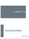
Quy mô fleet biến các lỗi thành phần hiếm gặp thành các sự kiện hệ thống thường xuyên.
Tuy nhiên, sự thành thạo luôn đi kèm một cám dỗ lặp lại: tin rằng hiểu một hệ thống là hiểu trọn vẹn nó. Cám dỗ đó sinh ra những ngụy biện và cạm bẫy trình bày ngay sau đây, nơi sự tự tin vượt quá sự khiêm tốn.
Self-Check: Question
A single data center GPU has an estimated Mean Time To Failure (MTTF) of approximately 5.7 years (\(\approx 50,000\text{ hours}\)). If an engineering team scales a distributed foundation model training run across a cluster of \(1,024\) identical GPUs, what is the expected cluster Mean Time Between Failures (\(\text{MTBF}_{\text{cluster}}\)) assuming independent constant-hazard failures, and what operational requirement does this impose?
- \(\text{MTBF}_{\text{cluster}} \approx 48.8\text{ hours}\) (approx. \(2\text{ days}\)); because cluster failure rate scales linearly with GPU count (\(\text{MTBF} = \text{MTTF} / N\)), multi-week training runs will routinely encounter hardware faults, making automated checkpointing and fast localized recovery an operational necessity.
- \(\text{MTBF}_{\text{cluster}} \approx 5.7\text{ years}\); hardware reliability is independent of the number of active nodes in the cluster.
- \(\text{MTBF}_{\text{cluster}} \approx 50\text{ minutes}\); network packet loss causes the entire cluster to crash once per hour.
- \(\text{MTBF}_{\text{cluster}} \approx 5,800\text{ years}\); distributed redundancy inherently increases total system reliability proportionally to cluster size.
How does the chapter demonstrate that ethical outcomes—such as accessibility, subgroup fairness, and environmental sustainability—are direct consequences of technical engineering decisions rather than abstract policy add-ons?
- Ethical concerns are external legal constraints that have no interaction with compiler flags, quantization formats, or model architecture.
- Engineering decisions—such as selecting high-precision floating-point formats (increasing datacenter carbon emissions), requiring multi-GPU nodes for inference (restricting deployment accessibility), or training on uncurated data (amplifying demographic bias)—directly dictate societal and ethical impacts.
- Model compression is purely a financial optimization that has no relationship to democratizing AI access.
- Algorithmic fairness can be fully guaranteed simply by omitting demographic feature columns from the raw dataset.
The chapter synthesizes the central insight that artificial intelligence is an ____ property that arises from the co-design and integration of data pipelines, neural architectures, hardware accelerators, serving runtimes, and governance frameworks, rather than from any single algorithmic insight.
True or False: Scaling an ML system from a single-node accelerator to a 1,024-node distributed training cluster invalidates the Iron Law of ML Systems, requiring engineers to discard single-node physical bounds in favor of purely empirical heuristics.
When moving from single-node ML systems to fleet-scale distributed systems, explain how the resource boundaries shift while the underlying physical laws remain invariant.
Ngụy biện và Cạm bẫy
Các ngụy biện và cạm bẫy trong hệ thống ML thường xuất phát từ một nguồn chung: coi hệ thống có thể tách thành các phần độc lập. Mỗi ngụy biện giả định rằng tối ưu một chiều, một chỉ số hoặc một giai đoạn là đủ; mỗi cạm bẫy cho thấy hậu quả khi giả định đó va chạm với thực tế vận hành.
Ngụy biện: Sự phức tạp của kỹ thuật hệ thống sẽ biến mất nhờ công cụ và lớp trừu tượng tốt hơn.
Các công cụ trừu tượng hoá sự phức tạp; chúng không loại bỏ các ràng buộc vật lý. Một framework cấp cao dù ẩn đi quản lý bộ nhớ thì vẫn tiêu tốn bộ nhớ. Một hệ thống AutoML tinh chỉnh siêu tham số vẫn phải đối mặt với biên Pareto. Đơn giản hóa một giao diện có thể chuyển gánh nặng sang chỗ khác, dù thiết kế tốt cũng có thể loại bỏ những phức tạp không cần thiết. Kỹ sư tin rằng công cụ có thể loại bỏ hoàn toàn các ràng buộc cơ bản sẽ bất ngờ khi những ràng buộc này tái xuất hiện ở quy mô lớn, thường dưới dạng còn khó chẩn đoán hơn cả vấn đề ban đầu.
Cạm bẫy: Tối ưu hóa một chỉ số mà không theo dõi các chi phí bị đẩy sang chỗ khác.
Khi một tối ưu hóa giúp giảm độ trễ 50%, hãy hỏi xem những phần khác đã thay đổi gì. Lượng tử hoá có thể làm tăng gánh nặng xác thực. Bộ nhớ đệm có thể đánh đổi dung lượng bộ nhớ để lấy tốc độ phục vụ (serving). Một số cách đơn giản hóa giúp loại bỏ những phức tạp không cần thiết; số khác lại đẩy chi phí sang chỗ khác. Những kỹ sư chỉ ăn mừng tăng trưởng ở một chỉ số mà không truy vết các tác động phụ có thể khiến hệ thống thất bại theo những cách khó lường. Việc đo lường sẽ quyết định điều gì đã xảy ra.
Ngụy biện: Thành thạo từng thành phần riêng lẻ không đồng nghĩa với việc thành thạo toàn bộ hệ thống.
Hiểu sâu về từng thành phần là cần thiết nhưng chưa đủ. Một kỹ sư chỉ hiểu các pipeline dữ liệu, quá trình huấn luyện, phục vụ (serving) và vận hành như những mảng riêng biệt sẽ vẫn gặp khó khăn với các hệ thống phức tạp, nơi một thay đổi trong lược đồ dữ liệu có thể lan sang huấn luyện, làm hỏng các giả định lượng tử hoá và gây suy giảm độ chính xác âm thầm trong môi trường sản xuất. Việc tích hợp có thể tạo ra sự phức tạp lớn hơn nhiều so với khi xem xét từng thành phần riêng lẻ, vì các giao diện làm tăng số kiểu lỗi có thể xảy ra. Tư duy hệ thống nghĩa là hiểu cách các thành phần tương tác với nhau, không chỉ cách chúng hoạt động riêng lẻ.
Cạm bẫy: Mở rộng quy mô thu thập dữ liệu mà không đo lường giá trị thông tin biên.
Niềm tin trực giác rằng “càng nhiều dữ liệu thì mô hình càng tốt” rất dễ thuyết phục, vì thường đúng ở giai đoạn đầu phát triển mô hình. Lựa chọn dữ liệu đã cho thấy quy luật lợi suất giảm dần có thể xuất hiện khi một tập dữ liệu đã đủ độ bao phủ: vượt ngưỡng này, dù tăng gấp đôi kích thước tập dữ liệu cũng chỉ cải thiện độ chính xác đôi chút, trong khi chi phí lưu trữ, tiền xử lý và gán nhãn lại tăng. Nguyên tắc trọng lực dữ liệu khuyến nghị đo lường các chi phí phía sau đó, bao gồm việc di chuyển hoặc quét lặp lại một tập dữ liệu lớn có đắt hơn so với đưa tài nguyên tính toán lại gần dữ liệu hay không. Kỹ sư tăng quy mô dữ liệu mà không đo lường lợi ích gia tăng trên mỗi mẫu đang tối ưu hóa sai biến.
Ngụy biện: Chỉ một chỉ số độ chính xác là đủ để đánh giá chất lượng mô hình.
Một mô hình chỉ được đánh giá bằng độ chính xác thì giống như đang sống trong một thế giới đơn chiều. Phân tích Pareto cần xét thêm độ trễ, thông lượng, bộ nhớ, năng lượng, tính công bằng và chi phí, sau khi đã chuẩn hóa hướng tối ưu của các mục tiêu. Với yêu cầu SLO về độ trễ đuôi 100 ms, một mô hình đạt 95% độ chính xác nhưng có 500 ms là không khả thi, trong khi mô hình 93% độ chính xác ở 50 ms vẫn là ứng viên. Nếu không có yêu cầu như vậy, không điểm nào mặc nhiên tốt hơn. Kỹ thuật có trách nhiệm cũng chỉ ra rằng độ chính xác tổng thể có thể che khuất chênh lệch lớn về tỷ lệ lỗi giữa các nhóm nhân khẩu học, nên ngay cả khía cạnh độ chính xác cũng phải được đo tách biệt theo nhóm. Việc đánh giá cần bao quát toàn bộ bề mặt Pareto liên quan, không chỉ một trục duy nhất.
Cạm bẫy: Coi mọi cảnh báo drift là tín hiệu để tự động rollback.
Phát hiện drift nên kích hoạt phản ứng đã được chẩn đoán, không phải rollback vô điều kiện. Rollback chỉ phù hợp khi đã xác định có thoái lui giữa các phiên bản hoặc bản phát hành. Drift phân phối từ bên ngoài sẽ không được sửa bằng cách khôi phục lại cùng một mô hình cũ; các hành động tự động an toàn hơn có thể là cảnh báo, fallback, giảm lưu lượng, hoặc tạm giữ dự đoán để xem xét, rồi thu thập dữ liệu và huấn luyện lại khi bằng chứng kết quả ủng hộ. Thiếu các cơ chế phản ứng theo từng nguyên nhân, sự suy giảm chất lượng có thể kéo dài cho tới khi có người phát hiện. Vì vậy, Vận hành machine learning gắn giám sát với hành động, nhưng hành động phải theo nguyên nhân đã chẩn đoán chứ không chỉ theo tín hiệu drift.
Ngụy biện: Chỉ cần tối ưu một giai đoạn của pipeline là hệ thống sẽ nhanh.
Định luật Amdahl (nguyên tắc 8) áp dụng trực tiếp cho các pipeline ML end-to-end. Tối ưu độ trễ suy luận trên bộ tăng tốc bằng 10× chỉ mang lại tốc độ toàn hệ thống 1.1× nếu phần tiền xử lý bị giới hạn bởi CPU chiếm 90 percent tổng độ trễ end-to-end — các phần tuần tự có thể phát sinh từ tăng cường hình ảnh phía máy chủ, tra cứu kho đặc trưng đồng bộ, hoặc token hóa vẫn chạy trên host trong một số triển khai. Quy luật sắt của hệ thống ML (nguyên tắc 3) phân tách thời gian thực thi thành các thành phần di chuyển dữ liệu, tính toán và độ trễ, để kỹ sư xác định thành phần chi phối trước khi đầu tư tối ưu. Benchmarking đã chính thức hóa quy trình chẩn đoán này thông qua các phương pháp profiling đo xem thời gian thực sự tiêu tốn ở đâu. Kỹ sư tối ưu mà không profiling là đang đoán mò, và Định luật Amdahl không khoan nhượng với những phỏng đoán nhắm sai thành phần.
Cạm bẫy: Chỉ profiling giai đoạn trông dễ tối ưu hóa nhất.
Các nhóm thường profiling lõi mô hình vì nó dễ thấy, dễ đo lường và do nhóm ML sở hữu, trong khi đường dẫn dữ liệu xung quanh lại bị chia nhỏ qua lưu trữ, tiền xử lý, mạng và mã ứng dụng. Góc nhìn cục bộ đó có thể khiến việc cải thiện lõi mô hình 10\(\times\) trông có vẻ cấp bách, ngay cả khi nó hầu như không thay đổi gì đường đi mà người dùng thấy. Profiling end-to-end giúp mục tiêu tối ưu hóa “trung thực”: giai đoạn cần cải thiện là giai đoạn đang giới hạn hệ thống, chứ không phải giai đoạn có bộ benchmark sạch sẽ nhất.
Tất cả tám ngụy biện và cạm bẫy đều có chung một gốc rễ: cám dỗ giản lược hệ thống thành các phần rời, dù bằng cách tối ưu một chỉ số, một giai đoạn, hay một thời điểm. Phần tóm tắt cuối cùng chống lại cách nhìn đó bằng việc quay về góc nhìn tích hợp: tư duy vượt qua ranh giới giữa các thành phần là kỷ luật cốt lõi của kỹ thuật hệ thống ML.
Self-Check: Question
An engineer profiles an image classification serving pipeline and finds that host CPU-bound image decoding, resizing, and normalization consume 90% of end-to-end request latency (\(f_{\text{serial}} = 0.90\)), while GPU neural network inference consumes the remaining 10% (\(f_{\text{accelerated}} = 0.10\)). The engineer rewrites the GPU kernel to achieve a \(10\times\) inference speedup (\(S = 10\)). What is the resulting overall system-level speedup, and which systems principle explains this outcome?
- \(10.0\times\) overall speedup; accelerator improvements dominate user-perceived performance.
- \(5.5\times\) overall speedup; system improvement is the average of the two pipeline stage speedups.
- \(0.90\times\) overall speedup; kernel compilation overhead causes net performance regression.
- Approximately \(1.10\times\) (or \(1.11\times\)) overall speedup; according to Amdahl’s Law, the unaccelerated 90% serial preprocessing fraction strictly caps end-to-end speedup to \(\text{Speedup} = \frac{1}{0.90 + \frac{0.10}{10}} = \frac{1}{0.91} \approx 1.10\times\).
A team selects Model Alpha over Model Beta because Alpha achieves 94.8% top-1 accuracy on a static benchmark versus Beta’s 93.2%. When deployed, Model Alpha violates the 100 ms P99 serving latency SLO by taking 420 ms, consumes \(4\times\) more memory, and exhibits a 16% error rate on an underrepresented user demographic. Which systems concept explains why single-metric evaluation led to this production failure?
- The Pareto Frontier; production ML systems operate across a multi-dimensional objective space (accuracy, tail latency, memory, energy, cost, and subgroup fairness), where optimizing aggregate accuracy in isolation can select an infeasible, costly, or discriminatory operating point.
- The Silicon Contract; models with higher accuracy automatically violate hardware execution contracts.
- Data Gravity; higher accuracy models physically pull network packets away from edge caches.
- Amdahl’s Law; aggregate accuracy scales inversely with the number of parallel workers.
True or False: High-level software frameworks, AutoML tools, and compiler abstractions eliminate underlying physical ML systems constraints (such as memory bandwidth bottlenecks, thermal dissipation limits, and Amdahl’s Law ceilings), allowing software engineers to ignore low-level hardware characteristics.
A production drift alarm fires due to seasonal changes in user shopping patterns. Explain why triggering an automated rollback to a model checkpoint trained three months earlier is an operational pitfall, and state the appropriate remediation.
Looking across all eight fallacies and pitfalls detailed in the chapter (tools hiding complexity, single-metric optimization, component-only mastery, unmeasured data scaling, unconditional rollbacks, and unprofiled stage optimization), identify the shared intellectual root cause that unites them and state the corrective systems engineering posture.
Tóm tắt
Kỹ thuật hệ thống ML khác với tối ưu hóa từng thành phần riêng lẻ ở chỗ nó đòi hỏi suy luận vượt qua các ranh giới. Mười ba nguyên tắc, quy tắc kinh nghiệm “bảo toàn độ phức tạp” và framework “hành trình hải đăng” cung cấp các công cụ phân tích để nhìn hệ thống như một tổng thể. Các giả định được nêu rõ giúp phân biệt rành mạch giữa các giới hạn chính xác với các mô hình được hiệu chỉnh, các chính sách SLO và các quy tắc kinh nghiệm thiết kế, nhờ đó các công cụ này vẫn hữu ích ngay cả khi các framework, thế hệ phần cứng và họ mô hình thay đổi.
Key Takeaways: Suy luận xuyên ranh giới
- Các giả định có ý nghĩa quan trọng trong các triển khai khác nhau: Mười ba nguyên tắc chuyển kỹ nghệ đặc thù của từng framework thành suy luận có thể đo lường, bằng cách kết hợp các giới hạn vật lý, phép phân tách, các mô hình được hiệu chỉnh, yêu cầu và các quy tắc kinh nghiệm. Chỉ áp dụng mỗi nguyên tắc trong đúng phạm vi đã nêu.
- Theo dõi các chi phí bị dịch chuyển mà không giả định sự bảo toàn: Nén, batch, giám sát và quản trị có thể chuyển gánh nặng giữa dữ liệu, thuật toán và máy, trong khi một thiết kế tốt có thể loại bỏ hoàn toàn độ phức tạp phát sinh ngoài ý muốn. Việc đo lường sẽ giúp phân biệt hai trường hợp này.
- Các ranh giới giúp ta nhận diện điểm nghẽn: Trong mô hình lý tưởng với batch 1 và hai GPU H100, giới hạn dưới của truyền dữ liệu qua bộ nhớ cho một token của mô hình Llama 2 70B là khoảng 295.2× so với giới hạn dưới theo khả năng tính toán đỉnh, và độ trễ p99 mang tính minh họa là 40× so với giá trị trung bình. Tư duy hệ thống nghĩa là đo lường chính xác nơi các yếu tố vật lý, lưu lượng và người dùng tạo ra ràng buộc.
- Quy mô làm thay đổi yếu tố ràng buộc: Bước tiến tiếp theo là quy mô lớn, nơi một cụm nghìn GPU biến thời gian sống trung bình của một thành phần (MTTF) kéo dài nhiều năm thành thời gian sống trung bình của cả cụm (MTBF) chỉ còn vài ngày. Các quy luật vật lý vẫn vậy, nhưng ràng buộc chuyển sang cấp độ đội máy.
Cuốn Computer Architecture: A Quantitative Approach của Hennessy và Patterson đã góp phần thiết lập một ngôn ngữ phân tích chung để so sánh CPI, tốc độ xung nhịp và số lượng lệnh (Hennessy and Patterson 2011; Hennessy and Patterson 2017). Tập hợp này cũng mong muốn đóng vai trò tương tự trong kỹ thuật hệ thống ML, dù không khẳng định rằng mọi chẩn đoán đều là bất biến. Đây là một khởi đầu, chứ không phải điểm kết thúc. Các nghiên cứu trong tương lai sẽ tiếp tục tinh chỉnh các mô hình, giả định và phạm vi.
Điều sẽ còn mãi là tư duy mà những nguyên tắc này thể hiện: suy luận dựa trên bằng chứng và các giới hạn vật lý thay vì chỉ phản ứng với triệu chứng; định lượng các đánh đổi thay vì chạy theo trào lưu; và coi thiết kế như một bài toán tối ưu hóa có ràng buộc. Đây là hệ quả kỹ thuật của bài học cay đắng mà phần giới thiệu đã rút ra từ bảy thập kỷ nghiên cứu AI: vì các phương pháp tổng quát có thể mở rộng theo năng lực tính toán liên tục vượt trội so với chuyên môn làm thủ công, nên lợi thế bền vững thuộc về kỹ thuật hệ thống có khả năng hấp thụ năng lực tính toán đó, chứ không phải bất kỳ một kiến trúc khéo léo đơn lẻ nào (Sutton 2019). Các framework cụ thể sẽ nổi lên rồi lụi tàn, các thế hệ phần cứng sẽ thay đổi, và kiến trúc mô hình sẽ bị thay thế. Nhưng suy luận có kỷ luật về dữ liệu, tính toán và các ràng buộc vật lý thì không.
Ở ngưỡng quy mô tiếp theo, một số mô hình không còn chạy vừa trên một máy, lỗi trở nên rất có khả năng xảy ra trên cả dàn máy, và các liên kết mạng có thể trở thành ràng buộc, bên cạnh bus bộ nhớ cục bộ. Vật lý không đổi; chỉ có quy mô mà tại đó nó trở thành ràng buộc là thay đổi.
Thế giới đang vội vã xây dựng các hệ thống AI. Nhiệm vụ của chúng ta là xây dựng chúng theo nguyên tắc kỹ thuật.
GS. Vijay Janapa Reddi, Đại học Harvard
Self-Check: Question
The summary emphasizes that the thirteen principles must be applied strictly within their stated assumptions and epistemic categories. Which of the following correctly categorizes these tools into exact physical/mathematical bounds, assumption-dependent fitted models, and product/governance policy requirements?
- All thirteen principles are universal physical conservation laws that hold unconditionally across all hardware, algorithms, and software frameworks.
- The Latency Budget is an unyielding law of physics, while Arithmetic Intensity and Amdahl’s Law are subjective product policy choices.
- Statistical Drift is a deterministic mathematical equation that guarantees exact accuracy loss under any dataset shift.
- The Iron Law, Arithmetic Intensity Law, and Amdahl’s Law are exact physical/mathematical bounds; Statistical Drift and Bias Feedback are assumption-dependent local fitted models; the Latency Budget and Verification Gap are product SLO and governance policy requirements.
How does the ‘Bitter Lesson’ of AI history—which observes that general computational scaling consistently outpaces human-crafted domain heuristics—reinforce the foundational importance of ML systems engineering?
- Handcrafted feature engineering and domain heuristics will always outperform compute-heavy neural networks.
- Algorithmic breakthroughs render hardware efficiency, memory bandwidth, and distributed coordination irrelevant.
- Because general algorithms that leverage massive computation consistently win over time, the durable competitive advantage belongs to systems engineering that can efficiently supply, orchestrate, and absorb that computation across silicon, memory, and networks.
- Systems engineering is only valuable when compute resources are severely constrained.
The conclusion draws an analogy between this textbook’s quantitative framework and Hennessy and Patterson’s foundational work in computer architecture, titled Computer Architecture: A ____ Approach, which transformed architecture from ad-hoc craft into a rigorous, measurable discipline.
Order the following steps in applying the quantitative principles across the ML system engineering lifecycle from foundational physical bounds to production operational monitoring:
- Operational Policy & Drift (Validating statistical drift diagnostics and verifying latency SLO budgets in production)
- Hardware Silicon Contract (Evaluating the roofline ridge point and arithmetic intensity against accelerator specifications)
- Pareto Trade-off Navigation (Applying compression and pruning to navigate the multi-objective efficiency frontier)
- Foundational Data Placement (Applying data-as-code and data gravity to determine storage and compute locality)
- Summarize what it means to ‘reason across boundaries’ in ML systems engineering, using an end-to-end example where an upstream data engineering decision propagates through framework lowering, hardware execution, and production drift monitoring.
Self-Check Answers
Self-Check: Answer
A production image classifier deployed across a mobile device fleet shows a 4-percentage-point drop in accuracy on specific handset cohorts. The weights file is unchanged, the compression team verified INT8 kernel speedups, and the serving team confirmed a P99 latency of 48 ms (under the 50 ms SLO). Which diagnostic posture is most consistent with the ‘system is the model’ thesis?
- Focus the investigation exclusively on serving execution, because runtime inference is the only stage operating during production.
- Trace the interaction between INT8 quantization scaling factors and firmware-specific image preprocessing paths, because production behavior is defined by the weights combined with the data pipeline, runtime hardware, and monitoring loop.
- Escalate to the architecture team to train wider convolutional layers, because an unchanged weights file implies that any remaining error must stem from model capacity.
- Treat the 4-point regression as acceptable random noise, because all engineering teams independently satisfied their local component metrics and the aggregate P99 latency is within budget.
Answer: The correct answer is B. Trace the interaction between INT8 quantization scaling factors and firmware-specific image preprocessing paths, because production behavior is defined by the weights combined with the data pipeline, runtime hardware, and monitoring loop. The central thesis of ML systems engineering is that ‘the system is the model’: the weights file is merely one component of a pipeline that includes data ingest, preprocessing, quantization scaling, hardware runtime execution, and drift monitoring. In the chapter’s mobile deployment case study, no single component failed in isolation; rather, a subtle coupling between INT8 quantization assumptions and device-specific image preprocessing firmware caused the localized accuracy loss. Escalating solely to architecture ignores the physical substrate; dismissing the drop as noise ignores cohort-specific degradation; and blaming only the serving runtime overlooks upstream preprocessing and quantization interactions.
Learning Objective: Apply the ‘system is the model’ thesis to diagnose a production regression that emerges from cross-layer interactions between preprocessing, quantization, and hardware runtimes.
A production recommender workload is dominated by terabyte-scale embedding tables where engineers spend significant effort deciding where data physically resides across storage tiers rather than optimizing dense matrix math. Which Lighthouse model embodies this constraint regime, and how does its primary bottleneck differ from low-batch GPT-2/Llama decoding?
- MobileNetV2; it is capacity-bound on microcontrollers, whereas autoregressive decoding is latency-bound by network packet round-trip times.
- ResNet-50; it is capacity-bound by image batch activation footprints in host DRAM, whereas LLM decode is compute-bound.
- Keyword Spotting (KWS); it is capacity-bound by microcontroller flash storage, whereas LLM decode is strictly compute-bound by tensor core peak FLOP/s.
- DLRM; it is capacity-bound by terabyte-scale embedding tables requiring physical data placement design, whereas low-batch LLM decode is memory-bandwidth-bound due to streaming weights with minimal arithmetic reuse per token.
Answer: The correct answer is D. DLRM; it is capacity-bound by terabyte-scale embedding tables requiring physical data placement design, whereas low-batch LLM decode is memory-bandwidth-bound due to streaming weights with minimal arithmetic reuse per token. The five Lighthouse models represent distinct binding regimes across the systems spectrum: DLRM is capacity-bound because terabyte-scale embedding tables cannot fit in GPU HBM, forcing distributed sharding across host RAM and SSDs; low-batch autoregressive LLM decoding is bandwidth-bound because weights must be read from HBM for every token with an arithmetic intensity of \(\approx 1\text{ FLOP/byte}\); ResNet-50 at large batch sizes is compute-bound; MobileNetV2 operates under mobile battery/thermal envelopes; and KWS operates under sub-megabyte SRAM and milliwatt constraints. The other options misclassify the workloads and their binding physical bottlenecks.
Learning Objective: Classify diverse ML workloads by their binding physical constraints (capacity-bound vs. bandwidth-bound vs. compute-bound) using the Lighthouse model framework.
**Order the following phases of the MobileNetV2 Lighthouse Journey in their chronological lifecycle order as constraints propagate from initial requirements through deployment operations:
- Compression (INT8 quantization navigating the Pareto frontier)
- Acceleration (Mapping operators to mobile NPUs under the Silicon Contract)
- Foundations (Establishing battery, thermal, and machine constraints)
- Architecture (Depthwise separable convolutions reducing FLOPs)
- Operations (Cohort-level drift monitoring across heterogeneous devices)
- Serving (Enforcing P99 latency budgets under 50 ms)**
Answer: The correct order is (3) -> (4) -> (1) -> (2) -> (6) -> (5).
Step-by-step lifecycle propagation: 1. (3) Foundations: Establishes the physical battery, thermal, and memory envelope of the edge device. 2. (4) Architecture: Designs depthwise separable convolutions to reduce arithmetic FLOPs by \(\approx 8.7\times\). 3. (1) Compression: Applies INT8 post-training quantization to reduce weight byte traffic by \(4\times\) vs. FP32. 4. (2) Acceleration: Compiles and maps INT8 fused operators onto mobile NPUs (e.g., Apple Neural Engine). 5. (6) Serving: Optimizes runtime image preprocessing to satisfy the P99 \(< 50\text{ ms}\) latency budget. 6. (5) Operations: Deploys continuous monitoring to detect accuracy drift across device cohorts and lighting conditions.
Learning Objective: Order the lifecycle phases of ML systems constraint propagation from foundational hardware constraints through architecture, compression, acceleration, serving, and operational monitoring.
True or False: If every engineering team in an ML organization independently satisfies its isolated component metric (e.g., architecture achieves an \(8.7\times\) FLOP reduction, compression achieves \(4\times\) weight reduction, and serving meets its P99 latency SLO), the integrated system is mathematically guaranteed to meet its end-to-end accuracy and correctness requirements in production.
Answer: False. Component correctness is necessary but insufficient for system correctness because ML systems exhibit complex cross-layer couplings across interfaces. An architectural change alters arithmetic intensity and operator support requirements; quantization introduces scaling factors and rounding errors; firmware-specific preprocessing pipelines may alter input color spaces or normalization; and serving dynamic batchers can alter tail latency distributions. When these components interact in production, subtle edge cases (such as quantization clipping on specific camera sensor firmware) create localized accuracy regressions that aggregate offline benchmarks and component-level SLOs never measure in isolation.
Learning Objective: Evaluate why component-level success metrics cannot guarantee end-to-end ML system correctness and reliability.
The conclusion argues that ‘the system is the model.’ Explain why treating the model solely as a static weights file (e.g., a 500 MB floating-point binary) fails in production, and define what constitutes the ‘true model.’
Answer: In production, model weights cannot function in isolation. The true model is the entire integrated pipeline: the data engineering pipeline that defines what features the model receives, the training infrastructure that determines what it learns, the serving runtime and hardware compiler that dictate how it executes, and the operational monitoring loop that tracks distribution drift. If upstream preprocessing changes or downstream hardware quantization clips values, model behavior degrades even if the weights file remains completely unchanged.
Learning Objective: Explain why production ML behavior is defined by the full end-to-end system rather than the weights file alone.
Self-Check: Answer
Consider serving one token at batch size 1 from a 70-billion-parameter Llama 2 model in FP16 (\(D_{\text{vol}} = 140\text{ GB}\), \(O \approx 140\text{ GFLOP}\)) sharded across two NVIDIA H100 GPUs (aggregate \(\text{BW} = 6.70\text{ TB/s}\), aggregate \(R_{\text{peak}} = 1,978\text{ TFLOP/s}\)). What are the idealized lower bounds for memory transfer (\(T_{\text{mem}}\)) and peak compute (\(T_{\text{comp}}\)), and what systems optimization strategy does this diagnostic dictate?
- Memory transfer time \(T_{\text{mem}} \approx 0.07\text{ ms}\) and compute time \(T_{\text{comp}} \approx 20.9\text{ ms}\); because compute time dominates by \(295\times\), the engineering team should prioritize hand-tuning tensor core matrix multiplication kernels.
- Memory transfer time \(T_{\text{mem}} \approx 2.09\text{ ms}\) and compute time \(T_{\text{comp}} \approx 2.09\text{ ms}\); because the workload operates exactly at the roofline ridge point, compute optimizations and memory optimizations provide identical returns.
- Memory transfer time \(T_{\text{mem}} \approx 20.9\text{ ms}\) and compute time \(T_{\text{comp}} \approx 0.07\text{ ms}\); because the memory bound is \(\approx 295\times\) larger than the compute bound, decode is heavily bandwidth-bound, meaning kernel FLOP tuning yields negligible speedup while batching and quantization directly reduce latency.
- Memory transfer time \(T_{\text{mem}} \approx 41.8\text{ ms}\) and compute time \(T_{\text{comp}} \approx 0.14\text{ ms}\); because sharding across two GPUs doubles the communication overhead, execution time increases by \(2\times\) relative to a single GPU.
Answer: The correct answer is C. Memory transfer time \(T_{\text{mem}} \approx 20.9\text{ ms}\) and compute time \(T_{\text{comp}} \approx 0.07\text{ ms}\); because the memory bound is \(\approx 295\times\) larger than the compute bound, decode is heavily bandwidth-bound, meaning kernel FLOP tuning yields negligible speedup while batching and quantization directly reduce latency. Applying the Iron Law and Arithmetic Intensity formulas: \(T_{\text{mem}} = \frac{140\text{ GB}}{6.70\text{ TB/s}} = \frac{140\text{ GB}}{6,700\text{ GB/s}} \approx 20.9\text{ ms}\), while \(T_{\text{comp}} = \frac{140\times 10^9\text{ FLOP}}{1,978\times 10^{12}\text{ FLOP/s}} \approx 0.07\text{ ms}\). The ratio \(\frac{T_{\text{mem}}}{T_{\text{comp}}} = \frac{20.9}{0.07} \approx 295\times\). Arithmetic intensity is \(\approx 1\text{ FLOP/byte}\), which lies far to the left of the H100 ridge point (\(I_{\text{ridge}} = \frac{1978\text{ TFLOP/s}}{6.7\text{ TB/s}} \approx 295\text{ FLOP/byte}\)). Under batch size 1, peak compute capacity is almost entirely idle while waiting for weights to stream from HBM. Optimizing compute kernels only shrinks the 0.07 ms term, whereas batching (reusing weights across requests) or weight quantization (halving bytes transferred) attacks the dominant 20.9 ms memory bottleneck. Inverting the values confuses compute with memory; claiming equal time misplaces the ridge point; and doubling execution time misapplies sharding.
Learning Objective: Calculate idealized memory-transfer and compute lower bounds for autoregressive token decoding and use arithmetic intensity to select high-leverage serving optimizations.
According to the Energy-Movement Invariant (\(E_{\text{total}} = \sum_j N_j E_j\)), accessing off-chip DRAM requires approximately 100 to 1,000 times more energy than executing a single FP16 or FP32 arithmetic operation. What is the direct systems design implication of this physical reality?
- Inference engines should prioritize minimizing total ALU operations above all else, even if intermediate tensors must be repeatedly written to and read from off-chip DRAM.
- Hardware accelerators consume identical energy regardless of whether memory accesses hit on-chip SRAM or off-chip DRAM, because memory controller power is fixed.
- Quantization saves energy exclusively by simplifying ALU multiplication logic, while memory traffic volume has negligible impact on total package power.
- Architectures and runtimes must maximize on-chip data reuse (e.g., via operator kernel fusion, SRAM tiling, and weight quantization), because eliminating off-chip DRAM round-trips yields orders-of-magnitude greater energy savings than reducing arithmetic FLOPs.
Answer: The correct answer is D. Architectures and runtimes must maximize on-chip data reuse (e.g., via operator kernel fusion, SRAM tiling, and weight quantization), because eliminating off-chip DRAM round-trips yields orders-of-magnitude greater energy savings than reducing arithmetic FLOPs. Moving bits across physical circuit board traces and off-chip memory buses (DRAM/HBM) consumes 100 to 1,000 times more energy (tens to hundreds of picojoules per access) than toggling transistors inside on-chip registers or arithmetic logic units (sub-picojoule per FLOP). Consequently, systems techniques that increase data locality—such as fusing pointwise operations into single kernels, tiling matrices to stay in SRAM caches, and quantizing weights to shrink memory footprint—derive the vast majority of their energy efficiency from avoiding DRAM traffic. The alternative claims contradict the physical reality of memory bus energy dissipation.
Learning Objective: Explain the physical basis of the Energy-Movement Invariant and evaluate how on-chip data reuse and kernel fusion minimize total system energy.
True or False: The conservation-of-complexity heuristic is an exact physical conservation law of computer science that proves every simplification in an ML pipeline interface creates an identical, mathematically equal compensating burden in another component.
Answer: False. The conservation-of-complexity heuristic (analogous to Tesler’s Law in UI design) is a diagnostic design heuristic, not an exact physical conservation law. While simplifying one interface often displaces work elsewhere (e.g., shorter user prompts shifting parsing and retrieval burdens into system prompts and vector lookups, or INT8 quantization adding validation burden), good engineering design can eliminate accidental complexity outright without creating equal compensating costs. Its value is diagnostic: prompting engineers to trace where validation, state, or operational burdens move after simplifying a component.
Learning Objective: Distinguish the conservation-of-complexity diagnostic heuristic from exact physical conservation laws.
The thirteen quantitative principles are unified by a central meta-heuristic known as the ____ heuristic, which reminds engineers that simplifying one interface often displaces validation, state, or operational burdens to another part of the system.
Answer: conservation of complexity (or conservation-of-complexity). The conservation-of-complexity heuristic serves as a diagnostic lens connecting Foundations, Build, Optimize, and Deploy. It prompts engineers to trace where costs land after optimizing or abstracting an individual component.
Learning Objective: Identify the conservation-of-complexity heuristic as the overarching diagnostic framework uniting the thirteen quantitative principles.
In the Cycle of ML Systems diagram (figure 1), the Deploy phase contains an explicit feedback arrow returning to Foundations (Data). Explain what production signals activate this feedback loop and why automated rollback is insufficient when the cause is external statistical drift.
Answer: The Deploy-to-Foundations feedback loop is activated by deployment diagnostics: the verification gap (estimating accuracy bounds under real traffic), statistical drift (distribution shifts in input features or user cohorts), training-serving skew (mismatched feature preprocessing paths), and bias feedback amplification. When a drift signal is detected, automated rollback only repairs software regressions caused by faulty code or bad model releases. If the underlying cause is external real-world distribution change (e.g., seasonal shifts, macro trends, or new user populations), rolling back to an older checkpoint trained on even staler data fails to restore accuracy. The feedback arrow requires diagnosing the root cause, collecting newly representative data, revalidating feature pipelines, and retraining or adapting the model.
Learning Objective: Analyze how deployment diagnostics (drift, skew, bias feedback) drive the feedback loop from production back to data engineering and retraining in the ML systems lifecycle.
Self-Check: Answer
A team chooses an ML framework primarily for its familiar Python syntax, only to discover months later that deploying the model to mobile NPUs and edge accelerators requires painful manual kernel rewrites because the framework lacks mature compiler lowering and graph optimization for those backends. Why does the Silicon Contract lens classify framework selection as an architectural commitment rather than an ergonomic preference?
- Frameworks embody fundamental architectural commitments to intermediate representations (IR), memory allocators, operator fusion passes, and backend compiler targets, which dictate whether the hardware’s peak efficiency can be realized downstream.
- Standard exchange formats such as ONNX are mathematically guaranteed to recover 100% of native hardware performance regardless of which framework was used during training.
- Frameworks operate exclusively as UI wrappers; hardware execution speed is determined solely by the neural network weights file.
- Modern hardware accelerators execute Python bytecode directly on silicon, so framework differences only affect model training time.
Answer: The correct answer is A. Frameworks embody fundamental architectural commitments to intermediate representations (IR), memory allocators, operator fusion passes, and backend compiler targets, which dictate whether the hardware’s peak efficiency can be realized downstream. Framework selection is a binding systems bet: each framework implements specific computation graphs, memory layout conventions, runtime dispatchers, and compiler backends (e.g., XLA, TorchDynamo, TensorRT). Choosing a framework without considering deployment targets can silently foreclose optimized lowering paths (such as INT8 quantization fusion or specialized NPU execution). Claiming that exchange formats recover full performance ignores operator dropping and loss of fusion metadata, while asserting that frameworks are mere UI wrappers misrepresents compiler execution stacks.
Learning Objective: Evaluate framework selection as an architectural commitment under the Silicon Contract that directly bounds downstream compiler lowering and hardware deployment efficiency.
A production serving dashboard for an interactive conversational assistant reports an average (mean) latency of 50 ms. However, user satisfaction metrics are declining, and detailed telemetry reveals a P99 tail latency of 2,000 ms (a \(40\times\) gap over the mean), violating the product SLO (\(T_{0.99} \le 200\text{ ms}\)). Which systems mechanism is a primary root cause of this massive tail spike in ML inference?
- Uniform degradation of memory bus bandwidth across all simultaneous client connections.
- A 40x increase in model weight parameters triggered dynamically whenever traffic surges.
- Heavy-tailed sequence lengths in autoregressive decoding, runtime garbage collection pauses in Python servers, and queueing delays caused by dynamic batching timeouts under bursty request arrivals.
- Deterministic floating-point underflow occurring on exactly one percent of input requests.
Answer: The correct answer is C. Heavy-tailed sequence lengths in autoregressive decoding, runtime garbage collection pauses in Python servers, and queueing delays caused by dynamic batching timeouts under bursty request arrivals. Mean latency severely hides tail behavior (\(P99 \gg \text{mean}\)). In ML serving, tail latency spikes stem from systems phenomena: variable-length prompt processing and generation loops in LLMs, garbage collection pauses in host runtimes, lock contention in dynamic batch schedulers, and queueing buildup when request arrival rates momentarily exceed processing capacity. Positing uniform bandwidth degradation describes a global slowdown rather than a tail quantile; dynamic parameter growth is technically nonsensical for static weights; and floating-point underflow confuses numerical precision with serving latency distributions.
Learning Objective: Analyze root causes of tail-latency spikes (\(P99 \gg \text{mean}\)) in production inference serving systems and evaluate them against latency budget SLOs.
True or False: Responsible AI metrics, such as subgroup error rates and bias feedback amplification, can be adequately handled as a post-hoc compliance audit after model serving is fully optimized, because fairness properties remain stable once offline validation passes.
Answer: False. Responsible AI is a dynamic systems engineering constraint governed by the same measurement discipline as latency and throughput. High aggregate accuracy on an offline benchmark can easily conceal massive error rate disparities on underrepresented demographic cohorts. In production, algorithmic predictions influence future data collection, creating compounding feedback loops (principle 13: \(\Delta_g(k) \ approx \Delta_g(0)\alpha_{\text{fb}}^k\)) that amplify historical bias over time. Treating fairness as an afterthought allows silent societal harms to compound undetected. Embedding disaggregated metrics, subgroup drift monitoring, and fairness validation directly into operational feature stores and serving pipelines ensures that regressions are detected and mitigated in real time.
Learning Objective: Justify why responsible AI monitoring and bias feedback mitigation are first-class operational systems constraints rather than post-hoc compliance audits.
An LLM training run encounters out-of-memory (OOM) errors during long-context training due to massive activation tensor footprints. Explain how Gradient Checkpointing (Activation Recomputation) resolves this bottleneck and identify the explicit systems trade-off it makes.
Answer: Gradient Checkpointing explicitly navigates the Iron Law by trading redundant compute for activation memory capacity. Instead of storing all intermediate layer activations during the forward pass, it discards them and recomputes them on-demand during the backward pass. This reduces peak activation memory footprint from \(\mathcal{O}(L)\) to \(\mathcal{O}(\sqrt{L})\) across layers at the cost of approximately 33% additional backward-pass FLOPs, allowing memory-bound long-context models to fit within GPU HBM.
Learning Objective: Analyze how gradient checkpointing trades compute FLOPs for activation memory capacity to solve memory-bound training bottlenecks.
Contrast the primary optimization objectives and time horizons of ML training systems versus interactive ML inference serving systems.
Answer: Training systems optimize for aggregate throughput (samples or tokens processed per second) over extended horizons of days to months, where large batches, high GPU utilization, and parallel scaling amortize overhead. In contrast, interactive inference systems optimize for strict tail-latency budgets (such as P99 or P99.9 latency in milliseconds) under dynamic, unpredictable user request arrivals, where low batch sizes, queuing delays, and cold-start overheads dominate the user experience.
Learning Objective: Compare the contrasting optimization objectives, batching regimes, and time horizons of training systems versus inference serving systems.
Self-Check: Answer
A compound ML service processes queries through a multi-stage pipeline: a vector retriever (50 ms), two specialized tools executed concurrently in parallel (Tool A takes 110 ms, Tool B takes 70 ms), an LLM generation step (180 ms), and a safety verifier (30 ms). Assuming negligible orchestration overhead, what is the theoretical request critical-path latency, and what new systems reliability challenge emerges compared to a single monolithic model?
- 440 ms (sum of all steps); each stage introduces strictly deterministic latency with zero risk of interface contract violations.
- 370 ms (\(50\text{ ms} + \max(110, 70)\text{ ms} + 180\text{ ms} + 30\text{ ms}\)); each interface introduces probabilistic failure modes (e.g., malformed JSON, schema drift, hallucinated tool calls) that require defensive validation, retry budgets, and composed reliability accounting.
- 180 ms; parallel execution across all components collapses total latency to the single slowest module.
- 110 ms; the critical path is bounded exclusively by the longest tool execution.
Answer: The correct answer is B. 370 ms (\(50\text{ ms} + \max(110, 70)\text{ ms} + 180\text{ ms} + 30\text{ ms}\)); each interface introduces probabilistic failure modes (e.g., malformed JSON, schema drift, hallucinated tool calls) that require defensive validation, retry budgets, and composed reliability accounting. On the critical path, parallel branches contribute their maximum rather than their sum: \(50 + \max(110, 70) + 180 + 30 = 50 + 110 + 180 + 30 = 370\text{ ms}\). Beyond latency, composed systems replace single monolithic model boundaries with multiple probabilistic interfaces. An LLM planner may produce schema deviations, tools may timeout, or verifiers may yield false rejections. Consequently, the system’s end-to-end reliability is the product of component reliabilities plus retry overheads, demanding defensive parsing, timeout budgets, and intermediate state observability. Summing all branches incorrectly adds parallel paths, while taking only the slowest module ignores serial dependencies.
Learning Objective: Calculate the critical-path latency of composed multi-component ML pipelines and analyze the probabilistic interface failure modes of compound AI systems.
When comparing a TinyML microcontroller deployment (e.g., Wake Vision on a Cortex-M core) with an H100 GPU cloud inference service, which statement correctly explains how the book’s quantitative framework applies across both extremes?
- TinyML is bounded solely by network socket latency, whereas cloud LLM serving is bounded entirely by CPU single-thread clock speed.
- TinyML eliminates the memory wall completely because microcontrollers have infinite SRAM access bandwidth.
- Both systems obey identical physical principles (the Iron Law, Arithmetic Intensity, and Silicon Contract), but their binding constraints diverge: TinyML is constrained by static SRAM/Flash capacity (\(<1\text{ MB}\)) and milliwatt power budgets, whereas low-batch cloud LLM decode is constrained by HBM memory bandwidth (\(3.35\text{ TB/s}\)).
- Cloud LLM inference operates with zero data movement overhead because H100 accelerators store all model weights permanently in ALU registers.
Answer: The correct answer is C. Both systems obey identical physical principles (the Iron Law, Arithmetic Intensity, and Silicon Contract), but their binding constraints diverge: TinyML is constrained by static SRAM/Flash capacity (\(<1\text{ MB}\)) and milliwatt power budgets, whereas low-batch cloud LLM decode is constrained by HBM memory bandwidth (\(3.35\text{ TB/s}\)). The quantitative principles are invariant across deployment scales separated by six orders of magnitude in power and memory. On a microcontroller, memory capacity (e.g., 256 KB SRAM) and strict energy envelopes prevent dynamic batching or large weights, forcing static memory pre-allocation and aggressive integer quantization. In cloud LLM serving, abundant compute is starved by the rate at which 140 GB of weights can be streamed across the HBM bus during batch-1 decode. The governing physics remains constant; only the active binding term shifts. The other choices contain physical and technical falsehoods regarding infinite SRAM, zero data movement, and socket bottlenecks.
Learning Objective: Compare how the Iron Law and Silicon Contract manifest across contrasting deployment regimes from TinyML microcontrollers to cloud accelerator clusters.
**An autonomous agent processes a complex user request across multiple specialized components. Order the execution stages along the request critical path from user query submission to final verified response:
- Safety & Factuality Verification (Defensive validation of response before delivery)
- Planner / Reasoner (Decomposing user intent and selecting tools)
- Output Generation (Synthesizing tool outputs into a coherent response)
- User Ingest & Retrieval (Vector search over external knowledge bases)
- Parallel Tool Execution (Querying external databases and specialized APIs)**
Answer: The correct order is (4) -> (2) -> (5) -> (3) -> (1).
Execution flow along the critical path: 1. (4) User Ingest & Retrieval: Ingests the query and performs vector retrieval to gather relevant context. 2. (2) Planner / Reasoner: Evaluates context and formulates a plan, generating structured tool call requests. 3. (5) Parallel Tool Execution: Concurrently executes external API queries, database lookups, or specialized domain models. 4. (3) Output Generation: An LLM synthesizes the tool outputs and retrieved context into a natural language response. 5. (1) Safety & Factuality Verification: Applies defensive guardrails, schema validation, and factuality checks before returning the response to the user.
Learning Objective: Order the critical-path stages of a compound AI request and identify the interface validation boundaries across retrieval, planning, tool execution, generation, and verification.
True or False: In safety-critical ML applications (such as clinical diagnostic imaging), if standard cloud infrastructure monitoring reports 99.99% uptime, HTTP 200 status codes, and sub-50 ms latencies, the deployment is guaranteed to be operating safely and correctly.
Answer: False. ML systems introduce silent failure modes where infrastructure availability dashboards remain completely green while the model produces clinically dangerous, incorrect predictions. Factors such as demographic covariate shift, changes in hospital imaging hardware, or subtle data pipeline format corruption alter predictive accuracy without triggering traditional HTTP, CPU, or memory errors. Operational safety requires continuous statistical drift detection, subgroup outcome auditing, calibrated uncertainty thresholds, and clinical review fallbacks.
Learning Objective: Analyze why traditional infrastructure uptime metrics fail to detect silent model degradation in safety-critical deployments.
Explain why robust AI design in safety-critical applications requires building explicit mechanisms for graceful degradation (such as uncertainty thresholds and fallback heuristics) rather than relying exclusively on pre-deployment validation.
Answer: Pre-deployment validation only tests finite samples from an assumed distribution and cannot guarantee correctness on out-of-distribution, adversarial, or shifted real-world inputs (the Verification Gap). Because neural networks can output confident but completely erroneous predictions, robust systems must design for graceful degradation at runtime. Concrete mechanisms include calibrated uncertainty estimation (triggering automated fallbacks to rule-based heuristics or human clinicians when confidence falls below safety thresholds), input sanity assertions, and defensive output validators. This bounds the blast radius of inevitable silent model failures.
Learning Objective: Design graceful degradation and fallback architectures for safety-critical ML systems operating under real-world uncertainty.
Self-Check: Answer
A single data center GPU has an estimated Mean Time To Failure (MTTF) of approximately 5.7 years (\(\approx 50,000\text{ hours}\)). If an engineering team scales a distributed foundation model training run across a cluster of \(1,024\) identical GPUs, what is the expected cluster Mean Time Between Failures (\(\text{MTBF}_{\text{cluster}}\)) assuming independent constant-hazard failures, and what operational requirement does this impose?
- \(\text{MTBF}_{\text{cluster}} \approx 48.8\text{ hours}\) (approx. \(2\text{ days}\)); because cluster failure rate scales linearly with GPU count (\(\text{MTBF} = \text{MTTF} / N\)), multi-week training runs will routinely encounter hardware faults, making automated checkpointing and fast localized recovery an operational necessity.
- \(\text{MTBF}_{\text{cluster}} \approx 5.7\text{ years}\); hardware reliability is independent of the number of active nodes in the cluster.
- \(\text{MTBF}_{\text{cluster}} \approx 50\text{ minutes}\); network packet loss causes the entire cluster to crash once per hour.
- \(\text{MTBF}_{\text{cluster}} \approx 5,800\text{ years}\); distributed redundancy inherently increases total system reliability proportionally to cluster size.
Answer: The correct answer is A. \(\text{MTBF}_{\text{cluster}} \approx 48.8\text{ hours}\) (approx. \(2\text{ days}\)); because cluster failure rate scales linearly with GPU count (\(\text{MTBF} = \text{MTTF} / N\)), multi-week training runs will routinely encounter hardware faults, making automated checkpointing and fast localized recovery an operational necessity. Under an independent constant-hazard model where any single GPU failure halts the synchronous training job, cluster failure rate is \(\lambda_{\text{cluster}} = \sum_{i=1}^N \lambda_{\text{gpu}} = 1024 \times \frac{1}{50,000\text{ hr}} \approx 0.02048\text{ failures/hr}\). Taking the inverse yields \(\text{MTBF}_{\text{cluster}} = \frac{50,000}{1024} \approx 48.8\text{ hours} \approx 2.03\text{ days}\). Over a 30-day training run, the cluster is statistically guaranteed to experience \(\approx 15\) hardware failure events. Fault tolerance—via asynchronous non-blocking checkpointing to persistent storage and rapid worker node replacement—becomes a mandatory systems requirement rather than an optional safeguard. The alternative choices misapply basic reliability scaling laws.
Learning Objective: Calculate cluster MTBF from component MTTF across large-scale accelerator pools and evaluate the operational necessity of fault tolerance and automated checkpointing.
How does the chapter demonstrate that ethical outcomes—such as accessibility, subgroup fairness, and environmental sustainability—are direct consequences of technical engineering decisions rather than abstract policy add-ons?
- Ethical concerns are external legal constraints that have no interaction with compiler flags, quantization formats, or model architecture.
- Engineering decisions—such as selecting high-precision floating-point formats (increasing datacenter carbon emissions), requiring multi-GPU nodes for inference (restricting deployment accessibility), or training on uncurated data (amplifying demographic bias)—directly dictate societal and ethical impacts.
- Model compression is purely a financial optimization that has no relationship to democratizing AI access.
- Algorithmic fairness can be fully guaranteed simply by omitting demographic feature columns from the raw dataset.
Answer: The correct answer is B. Engineering decisions—such as selecting high-precision floating-point formats (increasing datacenter carbon emissions), requiring multi-GPU nodes for inference (restricting deployment accessibility), or training on uncurated data (amplifying demographic bias)—directly dictate societal and ethical impacts. Technical choices inherently distribute costs and benefits: requiring high-end data center accelerators for serving excludes resource-constrained clinics from deploying medical AI (accessibility); unrepresentative data combined with feedback loops compounds disparities (fairness); and inefficient, uncompressed models increase Megawatt-hour datacenter power consumption and carbon footprints (sustainability). Ethics is an intrinsic dimension of technical design. The other options reflect discredited separation fallacies and naive fairness assumptions.
Learning Objective: Analyze how technical engineering decisions regarding efficiency, data curation, and energy consumption propagate directly into ethical, accessibility, and environmental consequences.
The chapter synthesizes the central insight that artificial intelligence is an ____ property that arises from the co-design and integration of data pipelines, neural architectures, hardware accelerators, serving runtimes, and governance frameworks, rather than from any single algorithmic insight.
Answer: emergent systems (or emergent). The text states that ‘intelligence is a systems property’—an emergent capability resulting from coordinating many components across the full D·A·M stack rather than an isolated mathematical breakthrough.
Learning Objective: Identify intelligence as an emergent systems property resulting from the co-design of data, models, hardware, and operational infrastructure.
True or False: Scaling an ML system from a single-node accelerator to a 1,024-node distributed training cluster invalidates the Iron Law of ML Systems, requiring engineers to discard single-node physical bounds in favor of purely empirical heuristics.
Answer: False. The fundamental physics of the Iron Law (\(T_{\text{seq}} = D_{\text{vol}}/\text{BW} + O/(R_{\text{peak}}\eta_{\text{hw}}) + L_{\text{lat}}\)) and the Silicon Contract remain invariant across all scales. However, the system resource boundaries expand: local GPU memory bandwidth is joined by inter-node network fabric bandwidth (e.g., InfiniBand/RoCE), device latency is joined by collective communication synchronization overheads (All-Reduce), and component reliability (MTTF in years) collapses into cluster-level MTBF (hours). The engineer applies the same quantitative bottleneck reasoning to this wider physical boundary.
Learning Objective: Explain why fundamental physical principles remain valid while resource boundaries expand during the transition from single-node to fleet-scale distributed systems.
When moving from single-node ML systems to fleet-scale distributed systems, explain how the resource boundaries shift while the underlying physical laws remain invariant.
Answer: Scaling from single-node to fleet scale does not change the governing physics—the Iron Law (\(T = D/\text{BW} + O/R_{\text{peak}} + L\)) still governs execution time—but the boundaries expand. Local memory bus bandwidth (HBM) is joined by cross-node network fabric bandwidth (InfiniBand/RoCE); single-device latency is joined by collective communication synchronization overhead (All-Reduce); single-GPU component MTTF (years) collapses into cluster MTBF (hours); and data gravity shifts from host-to-device transfers to cross-datacenter data placement. The engineer must apply the same quantitative bottleneck diagnosis across this wider boundary.
Learning Objective: Explain how fleet-scale distributed systems expand resource boundaries (networking, collective communication, cluster MTBF) while preserving fundamental physical invariants.
Self-Check: Answer
An engineer profiles an image classification serving pipeline and finds that host CPU-bound image decoding, resizing, and normalization consume 90% of end-to-end request latency (\(f_{\text{serial}} = 0.90\)), while GPU neural network inference consumes the remaining 10% (\(f_{\text{accelerated}} = 0.10\)). The engineer rewrites the GPU kernel to achieve a \(10\times\) inference speedup (\(S = 10\)). What is the resulting overall system-level speedup, and which systems principle explains this outcome?
- \(10.0\times\) overall speedup; accelerator improvements dominate user-perceived performance.
- \(5.5\times\) overall speedup; system improvement is the average of the two pipeline stage speedups.
- \(0.90\times\) overall speedup; kernel compilation overhead causes net performance regression.
- Approximately \(1.10\times\) (or \(1.11\times\)) overall speedup; according to Amdahl’s Law, the unaccelerated 90% serial preprocessing fraction strictly caps end-to-end speedup to \(\text{Speedup} = \frac{1}{0.90 + \frac{0.10}{10}} = \frac{1}{0.91} \approx 1.10\times\).
Answer: The correct answer is D. Approximately \(1.10\times\) (or \(1.11\times\)) overall speedup; according to Amdahl’s Law, the unaccelerated 90% serial preprocessing fraction strictly caps end-to-end speedup to \(\text{Speedup} = \frac{1}{0.90 + \frac{0.10}{10}} = \frac{1}{0.91} \approx 1.10\times\). Amdahl’s Law (principle 8) governs end-to-end ML pipelines. When 90% of execution time remains unaccelerated on the host CPU (e.g., JPEG decoding, tokenization, or database feature lookups), even an infinite (\(S = \infty\)) speedup on the GPU inference kernel would yield at most \(\frac{1}{0.90} \approx 1.11\times\) overall system speedup. Optimizing without profiling where time actually goes is guessing, and Amdahl’s Law severely penalizes optimizations that target the non-dominant term. The other options violate Amdahl’s Law arithmetic.
Learning Objective: Apply Amdahl’s Law to calculate end-to-end speedup when optimizing isolated pipeline stages and identify when unaccelerated preprocessing bounds system throughput.
A team selects Model Alpha over Model Beta because Alpha achieves 94.8% top-1 accuracy on a static benchmark versus Beta’s 93.2%. When deployed, Model Alpha violates the 100 ms P99 serving latency SLO by taking 420 ms, consumes \(4\times\) more memory, and exhibits a 16% error rate on an underrepresented user demographic. Which systems concept explains why single-metric evaluation led to this production failure?
- The Pareto Frontier; production ML systems operate across a multi-dimensional objective space (accuracy, tail latency, memory, energy, cost, and subgroup fairness), where optimizing aggregate accuracy in isolation can select an infeasible, costly, or discriminatory operating point.
- The Silicon Contract; models with higher accuracy automatically violate hardware execution contracts.
- Data Gravity; higher accuracy models physically pull network packets away from edge caches.
- Amdahl’s Law; aggregate accuracy scales inversely with the number of parallel workers.
Answer: The correct answer is A. The Pareto Frontier; production ML systems operate across a multi-dimensional objective space (accuracy, tail latency, memory, energy, cost, and subgroup fairness), where optimizing aggregate accuracy in isolation can select an infeasible, costly, or discriminatory operating point. Evaluating models solely along a single accuracy dimension inhabits a one-dimensional fantasy. In production, models must satisfy multi-objective constraints along the Pareto Frontier (principle 5): meeting P99 latency budgets (principle 12), fitting hardware memory capacity, respecting energy/cost limits, and ensuring equitable error rates across demographic subgroups (principle 13). A model with 1.6% higher aggregate accuracy that violates latency SLOs and exhibits extreme subgroup disparity is an engineering failure. The other options misapply unrelated systems concepts.
Learning Objective: Critique single-metric accuracy evaluation and apply the Pareto Frontier to assess production models across latency, memory, energy, and subgroup fairness.
True or False: High-level software frameworks, AutoML tools, and compiler abstractions eliminate underlying physical ML systems constraints (such as memory bandwidth bottlenecks, thermal dissipation limits, and Amdahl’s Law ceilings), allowing software engineers to ignore low-level hardware characteristics.
Answer: False. Tools and abstractions hide and manage complexity; they do not eliminate physical constraints. A framework that abstracts memory management still transfers bytes across physical buses and consumes memory capacity; an AutoML engine tuning hyperparameters still operates on the Pareto frontier; and a compiler optimizing GPU kernels remains strictly bounded by Amdahl’s Law and memory wall physics. Engineers who assume tools eliminate physical constraints are routinely surprised when those constraints resurface at scale as mysterious OOM errors, tail latency spikes, or thermal throttling.
Learning Objective: Analyze why software abstractions manage complexity rather than eliminating physical hardware constraints.
A production drift alarm fires due to seasonal changes in user shopping patterns. Explain why triggering an automated rollback to a model checkpoint trained three months earlier is an operational pitfall, and state the appropriate remediation.
Answer: Automated rollback is effective for software bugs or bad releases, but external real-world distribution drift cannot be repaired by restoring an older model trained on an even staler distribution. Restoring the older checkpoint will perform just as poorly or worse. The appropriate remediation is a diagnosed response: alerting the team, temporarily routing traffic to fallback heuristics or reducing traffic, collecting fresh ground-truth labels from the new distribution, and retraining/adapting the model.
Learning Objective: Differentiate between release regressions and external distribution drift to select appropriate operational remediations.
Looking across all eight fallacies and pitfalls detailed in the chapter (tools hiding complexity, single-metric optimization, component-only mastery, unmeasured data scaling, unconditional rollbacks, and unprofiled stage optimization), identify the shared intellectual root cause that unites them and state the corrective systems engineering posture.
Answer: The shared root cause is the reductionist temptation to treat an ML system as decomposable into independent, isolated parts—optimizing one dimension, one metric, one pipeline stage, or one moment in time as if the surrounding system were static. The corrective systems engineering posture is holistic boundary reasoning: measuring the end-to-end request path, profiling where time and bytes actually go before optimizing, tracing how decisions in one layer displace costs to other layers (conservation-of-complexity heuristic), and evaluating performance across the full multi-dimensional Pareto surface under real-world operational constraints.
Learning Objective: Synthesize the shared systems misconception (reductionism and isolated optimization) underlying common ML systems failures.
Self-Check: Answer
The summary emphasizes that the thirteen principles must be applied strictly within their stated assumptions and epistemic categories. Which of the following correctly categorizes these tools into exact physical/mathematical bounds, assumption-dependent fitted models, and product/governance policy requirements?
- All thirteen principles are universal physical conservation laws that hold unconditionally across all hardware, algorithms, and software frameworks.
- The Latency Budget is an unyielding law of physics, while Arithmetic Intensity and Amdahl’s Law are subjective product policy choices.
- Statistical Drift is a deterministic mathematical equation that guarantees exact accuracy loss under any dataset shift.
- The Iron Law, Arithmetic Intensity Law, and Amdahl’s Law are exact physical/mathematical bounds; Statistical Drift and Bias Feedback are assumption-dependent local fitted models; the Latency Budget and Verification Gap are product SLO and governance policy requirements.
Answer: The correct answer is D. The Iron Law, Arithmetic Intensity Law, and Amdahl’s Law are exact physical/mathematical bounds; Statistical Drift and Bias Feedback are assumption-dependent local fitted models; the Latency Budget and Verification Gap are product SLO and governance policy requirements. A vital insight of the chapter is that not all principles have identical epistemic status. The Iron Law, Arithmetic Intensity (roofline), and Amdahl’s Law are hard physical and mathematical limits dictated by hardware and execution structure. Statistical Drift and Bias Feedback are empirical, local models whose parameters (\(\lambda, \alpha_{\text{fb}}\)) must be fitted to measured outcome data. Latency Budgets (\(T_q \le L_{\text{budget}}\)) and the Verification Gap are product specifications and risk-tolerance policies. Treating fitted models or policies as universal physical invariants leads to faulty engineering conclusions. The other options misclassify these tools.
Learning Objective: Distinguish between exact physical bounds, assumption-dependent fitted models, and policy requirements within the thirteen quantitative principles framework.
How does the ‘Bitter Lesson’ of AI history—which observes that general computational scaling consistently outpaces human-crafted domain heuristics—reinforce the foundational importance of ML systems engineering?
- Handcrafted feature engineering and domain heuristics will always outperform compute-heavy neural networks.
- Algorithmic breakthroughs render hardware efficiency, memory bandwidth, and distributed coordination irrelevant.
- Because general algorithms that leverage massive computation consistently win over time, the durable competitive advantage belongs to systems engineering that can efficiently supply, orchestrate, and absorb that computation across silicon, memory, and networks.
- Systems engineering is only valuable when compute resources are severely constrained.
Answer: The correct answer is C. Because general algorithms that leverage massive computation consistently win over time, the durable competitive advantage belongs to systems engineering that can efficiently supply, orchestrate, and absorb that computation across silicon, memory, and networks. Rich Sutton’s Bitter Lesson notes that 70 years of AI research show that methods leveraging raw computation scale indefinitely, while specialized human-crafted heuristics plateau. The direct systems corollary is that building the infrastructure to deliver, feed, and manage that computation—high-throughput training clusters, memory-bandwidth-optimized inference runtimes, efficient communication topologies, and robust operations—is the true engine of sustained AI progress. The alternative choices contradict the Bitter Lesson and the systems synthesis.
Learning Objective: Synthesize the systems engineering corollary to the Bitter Lesson, explaining why infrastructure that scales computation provides the durable foundation of AI progress.
The conclusion draws an analogy between this textbook’s quantitative framework and Hennessy and Patterson’s foundational work in computer architecture, titled Computer Architecture: A ____ Approach, which transformed architecture from ad-hoc craft into a rigorous, measurable discipline.
Answer: Quantitative (or Quantitative Approach). Hennessy and Patterson’s Computer Architecture: A Quantitative Approach established the quantitative discipline (CPI, memory hierarchy formulas, Amdahl’s Law) that this textbook adapts to machine learning systems.
Learning Objective: Identify the historical analogy between the quantitative framework of ML systems engineering and Hennessy and Patterson’s Quantitative Approach to computer architecture.
**Order the following steps in applying the quantitative principles across the ML system engineering lifecycle from foundational physical bounds to production operational monitoring:
- Operational Policy & Drift (Validating statistical drift diagnostics and verifying latency SLO budgets in production)
- Hardware Silicon Contract (Evaluating the roofline ridge point and arithmetic intensity against accelerator specifications)
- Pareto Trade-off Navigation (Applying compression and pruning to navigate the multi-objective efficiency frontier)
- Foundational Data Placement (Applying data-as-code and data gravity to determine storage and compute locality)**
Answer: The correct order is (4) -> (2) -> (3) -> (1).
Step-by-step epistemic progression: 1. (4) Foundational Data Placement: Evaluates data gravity and data-as-code to anchor storage, ingestion, and compute locality. 2. (2) Hardware Silicon Contract: Analyzes the hardware roofline ridge point (\(I_{\text{ridge}} = R_{\text{peak}}/\text{BW}\)) and model arithmetic intensity to identify whether compute or memory bandwidth dominates. 3. (3) Pareto Trade-off Navigation: Explores the Pareto frontier using quantization, pruning, or distillation to balance precision, footprint, and throughput. 4. (1) Operational Policy & Drift: Establishes product SLO latency budgets (\(T_q \le L_{\text{budget}}\)), verifies statistical drift diagnostics, and monitors subgroup fairness in production.
Learning Objective: Order the systematic application of quantitative principles across the ML systems lifecycle from data foundations to hardware contract, optimization, and operational verification.
Summarize what it means to ‘reason across boundaries’ in ML systems engineering, using an end-to-end example where an upstream data engineering decision propagates through framework lowering, hardware execution, and production drift monitoring.
Answer: Reasoning across boundaries means analyzing an ML system as an interconnected whole where decisions in one layer constrain all others. For example: (1) In Data Engineering, choosing raw image formats and normalization ranges dictates input preprocessing volume; (2) In Architecture & Frameworks, this choice determines whether convolutions can be lowered to INT8 tensor cores; (3) In Hardware Acceleration, INT8 execution cuts DRAM traffic by \(4\times\), shifting the roofline operating point closer to compute saturation; (4) In Serving, this latency win unlocks headroom to satisfy the P99 SLO; and (5) In Operations, device-specific camera firmware shifts require subgroup drift monitoring to catch silent quantization clipping before it harms users. An engineer who understands only one layer cannot predict or debug this end-to-end propagation.
Learning Objective: Synthesize the core discipline of ML systems engineering: reasoning across data, algorithm, machine, serving, and governance boundaries.